Performance Variables

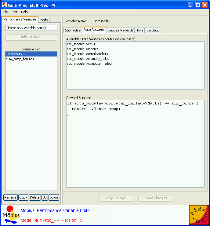
The Performance Variable Editor is shown in <xr id="fig:reward_main" />. It consists of a menu bar and a split pane. The left side of the split pane contains a tabbed panel with two tabs: Performance Variables and Model. The right side of the split pane contains the editable fields for the currently selected performance variable.

<xr id="fig:reward_main" nolink />: Performance Variable Editor.</figure>

The Performance Variables tab is the main display and is used to create new variables or select an existing variable so it can be edited, renamed, copied, or deleted.

The Model tab lists the top-level model on which this reward model is built. Often, the top-level model is a composed model, in which case the available submodels within the composed model are listed in the lower table. The top-level model is also referred to as child model of this reward model.

In addition to the menu options that are common to all Möbius editors (see Section 3.1), the following operations are available within the performance variable editor, via the main menu, buttons at the bottom of the left panel, or a right-click pop-up in the variable list:

Add Variable: Type the name of the new variable and click the Add Variable button (or hit the $<Enter>$ key). The text in the new variable name text field disappears automatically when you type the new variable name.

Rename: Change the name of the selected variable.

Move Up: Move a variable up in the variable list. Allows for the grouping of related variables.

Move Down: Move a variable down in the variable list. Allows for the grouping of related variables.

Copy: Copy the selected variable to a new variable with a new name.

Delete: Delete the selected variable.

Variable definition

When a variable is selected in the variable list, the right side of the editor displays the variable definition panel. At the top of this panel is the name of the variable currently selected. Beneath the name is a tabbed pane used to define specifics of the variable. The tabbed pane contains five tabs: Submodels, Rate Rewards, Impulse Rewards, Time, and Simulation.

Submodels

The Submodels tab lists the names of all of the models in the child of the reward model. You must apply each reward variable to one or more of the available submodels. You can do so by selecting the model in the list. The $<$ Ctrl $>$ key can be used to select multiple individual items. The $<$ Shift $>$ key can be used to select a range of items.

When Möbius computes the reward function, it will do so on each instance of the selected models. For example, if there are N instances of the selected submodel in the top-level model, the reward function will be evaluated N times. For some types of reward functions, it is desirable to divide the reward function by the number of instances in the model (N in this example), so that the reward represents the average of the N instances.

With the current version of Möbius, you must use caution when defining rewards that depend on the state of multiple submodels. When multiple instances of the specified submodels are created by replication in the composed model, the results obtained are often nonintuitive. For example, consider a child model that is a composed model with 2 instances of submodel “A” and 3 instances of submodel “B”. If a reward is defined on state variables from both A and B, one might expect that the function would be evaluated five times (once on each A, and once on each B). However, that is not the case. Instead, the function will be evaluated a total of 6 times, once for each possible pair of an A with a B. (This behavior might change in future versions of Möbius.)

Selecting the submodel populates the Available State Variables panel in the Rate Rewards tab with the names of all state variables found in the selected submodel(s). Similarly, it also populates the Available Actions panel in the Impulse Rewards tab with all of the actions found in the selected submodel(s).

Rate rewards

The Rate Rewards tab is used to define rewards based on the time in each state. The top panel lists the Available State Variables, based on the submodels selected in the Submodels tab. The bottom panel contains the Reward Function. The reward function defines the measurement this rate reward should take. The reward function is written as a piece of C++ code, and should end with a return statement returning the value of the function.

As a shortcut for the user, double-clicking in the top panel inserts the state variable name at the location of the text cursor in the bottom panel. The value of the reward must be returned using the state variable value access function. This function is formalism-specific. For example, the value access function is Mark() for places in SANs and buckets in Buckets and Balls. Refer to the appropriate formalism documentation for details on access functions and other available functions that could be used to define rewards.

Impulse rewards

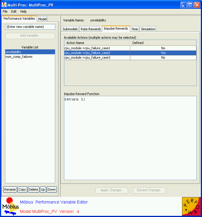
The Impulse Rewards tab defines reward functions that are evaluated when actions in the child model fire. The top panel contains a table showing the name of each action in the child model, and a column specifying whether or not an impulse function is defined for the action. To define an impulse function, click on the name of the function, and then write the C++ function for the impulse reward in the lower panel. The code should return the function result using the C++ return statement.

<xr id="fig:reward_impulse" nolink />: Impulse reward definition.</figure>

Impulse rewards can easily be used to count the number of times an action fires during an interval of time. To do so, set the impulse function to return 1, and set the type to Interval of Time with appropriate start and stop times (see next section).

Time

In order to solve for the reward measures via either simulation or numerical solution techniques, Möbius requires the specification of additional parameters for each reward variable. These parameters define the type of results to measure for the specific times of interest.

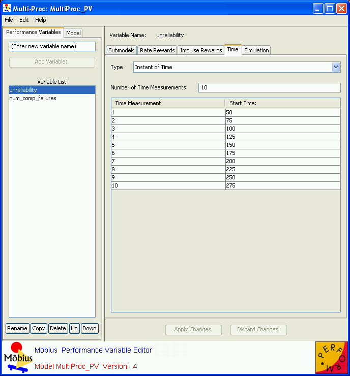
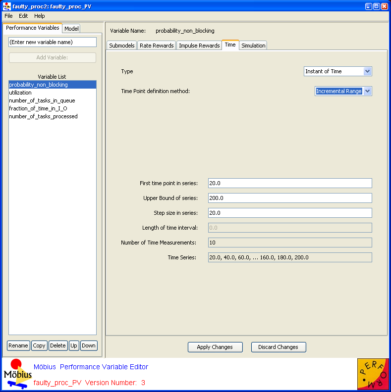
Reward variables can be defined as one of several different types. The type of the reward variable determines when, in system time, the reward function is evaluated. Evaluation times can be specified manually using a table, as shown in <xr id="fig:reward_time" />, or as an incremental range, as shown in <xr id="fig:reward_time_inc" />.

<xr id="fig:reward_time" nolink />: Manual selection of time points for instant of time variable.</figure>

<xr id="fig:reward_time_inc" nolink />: Definition of time points using incremental range options.</figure>

The possible reward variable types are:

Instant of Time: The reward function is evaluated at the specified point in time. The desired time is specified in the Start time field. Units of time are the same units used for the parameters for the action distributions in the atomic models.

Interval of Time: The variable returns the weighted sum of all of the values of the reward function, where each value is weighted by the amount of time the value is in existence, between the starting and ending times of the specified interval. The desired start and stop times for the interval are specified in the Start and Stop text fields.

Time Averaged Interval of Time: The variable returns the interval of time result, divided by the length of time for the interval. As with interval of time variables, the desired start and stop times for the interval are specified in the Start and Stop text fields.

Steady State: The reward function is evaluated after the system being modeled reaches steady state. The steady state simulation algorithm used is referred to in literature as batch means (see ^[1]). This approach assumes that there is an initial transient period that must pass before the system reaches its steady state behavior. Once the system is in steady state, the algorithm evaluates the reward function multiple times to gather the observations to compute the statistics. This technique is appropriate when enough time occurs between the samples to permit the assumption that the samples are independent of each other.

Simulation using batch means is typically more efficient than standard simulation approaches, since the possibly long initial transient period must be processed only once in batch means for all the observations, while traditional simulation would require processing of the initial transient period for each observation.

Simulation

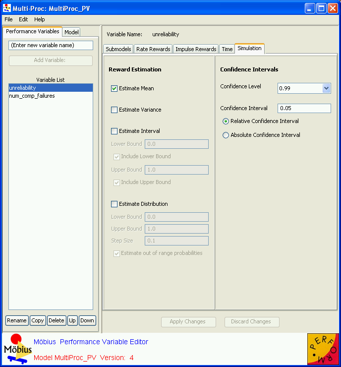
The Simulation tab is used to define two aspects of reward variables that are unique to simulation. They are variable estimation and confidence interval definition.

<xr id="fig:reward_sim" nolink />: Impulse reward definition.</figure>

Estimation

When a model is being solved via simulation, the system is executed multiple times using different randomly generated event streams. Each execution generates a different trajectory through the possible event space of the system, due to the differences in the order and choice of events that occur. The reward variables are evaluated for each trajectory to create an observation. Statistical estimates of the reward variable value are then computed from the observations.

Multiple estimates can be computed for each variable. Möbius supports four basic estimations: mean, variance, the probability that the function is in an interval, and the probability distribution (and density) functions. To enable the computation of any of these types, click the appropriate check box. Additional parameters are required for intervals and distributions.

When Estimate Interval is selected, the four interface components beneath it are enabled. The Lower Bound and Upper Bound fields are used to specify the lower and upper bounds of the interval. The Include Upper (Lower) Bound checkboxes determine whether the upper (lower) bound itself is part of the interval.

When Estimate Distribution is selected, the four interface components beneath it are enabled. The Lower Bound and Upper Bound text fields specify the lower and upper limits of the distribution that will be measured. The Step Size determines the width of each bin in the discrete representation of the distribution. The number of samples in the distribution is computed by $(Upper - Lower) / Step Size$ . Varying those three parameters makes it possible to focus distributions on specific areas of the reward function space, with varied resolutions. If Estimate out of range probabilities is selected, the probability that the reward function value will be lower than the lower bound of the distribution will be computed, as will the probability that the reward will be above the upper bound of the distribution.

Confidence

In order to get statistically significant estimations of the reward variables, it is necessary to generate many trajectories. In order to give an estimate of the accuracy of the calculated estimates, confidence intervals are computed as the observations are collected. When the simulation reaches the desired confidence level for every variable, the simulation will stop. (The simulator will also stop if it reaches a maximum observation limit without achieving the desired confidence level.)

Three parameters define the confidence interval. The Confidence Level text box specifies the desired probability that the exact value of the reward variable will be within the specified interval around the variable estimate. The Confidence Interval text box specifies the width of the acceptable interval around the variable estimate. The interval can either be Relative to the variable estimate, or be an Absolute number. For instance, a relative confidence interval of .1 and a confidence level of .95 for a mean variable will not be satisfied until the confidence interval is within 10% of the mean estimate 95% of the time.

References

↑ A. Law and W. D. Kelton. Simulation modeling and Analysis. McGraw-Hill, 1991.

[lawkelton:sim-1] A. Law and W. D. Kelton. Simulation modeling and Analysis. McGraw-Hill, 1991.

[1]

Performance Variables

Contents