Building Models

From Mobius Wiki
Revision as of 20:32, 7 May 2014 by Ctbucha2 (talk | contribs) (Elements)
(diff) ← Older revision | Latest revision (diff) | Newer revision → (diff)
Jump to: navigation, search

Contents

Project Manager

The Project Manager is the main console for Möbius and is shown in <xr id="fig:projman" />. Across the top is a main menu, with three menu categories: Project, Tools, and Help. The main display is a console view that shows messages for the operations performed by Möbius. Descriptions of the operations available under each menu category are presented in the following sections.


<figure id="fig:projman">

Projman.png


<xr id="fig:projman" nolink />: The Project Manager window.
</figure>


Project Menu

The Project menu contains several operations related to Möbius projects. A Möbius project is the fundamental unit of organization for each system model in Möbius. A project contains one or more models defining the system and instances, descriptions of what parameters to solve for, and instances of solvers to generate the solutions. More details on projects can be found in Section 2.

The Project menu contains the following operations:

  • New: Create a new project. A dialog will appear prompting for the new project name. After you enter a valid project name, the author, and a description. The author and description are optional and for informational purposes only. These two fields can be changed at a later date. The new project will be opened.
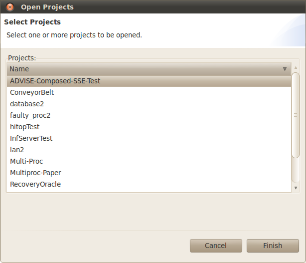
  • Open: Open an existing project. A dialog to select the project to open will appear as shown in <xr id="fig:project_dialog" />. You may select multiple projects to be opened simultaneously. You can quickly open a single project by double clicking it.


<figure id="fig:project_dialog">

Projman projdialog.png


<xr id="fig:project_dialog" nolink />: Use the project selection dialog to open projects.
</figure>


  • Copy: Copy an existing project to a new project. You must close the existing project to guarantee a stable copy.
  • Rename: Give an existing project a new name. You must close the project before it can be renamed.
  • Clean: Remove all temporary files from the project.
  • Resave: Regenerate all project source code and libraries. Resaving the project is required before a project is opened for the first time after a Möbius upgrade. You must also resave after unarchiving a project.
  • Delete: Delete the project. The most-recently-deleted project is stored in a “Deleted” folder within the Möbius project directory.
  • Archive: Create a backup of the project. After you select one or more projects, you will be asked for details about how you want each of the selected projects to be archived. After you specify the name of the archive file, you must select one of two options, Full archive and Minimal archive. A full archive includes all files found within the project. A minimal archive includes only the files necessary to define all models within the project. In a minimal archive, object files, libraries, executables, and results are not backed up. Minimal archives are helpful when multiple users are collaborating on the same model, since they create small archives that are convenient to email. The format for the archive is gzipped tar (.tgz) format.
  • Unarchive: Restore a project from an archive file. If the project to be restored has the same name as an existing project, you can either delete the existing project or cancel the restoration. Restoring one project on top of a different one could cause corruption and confusion, so is not supported. Unarchived projects should be resaved before they are used.
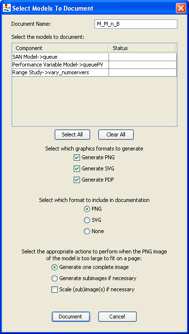
  • Document: Create HTML documentation for the chosen project. After you select the project to document, you use the Document Project dialog (see <xr id="fig:doc_proj" />) to select the models in the project that should be documented. Documentation is written to a subdirectory in the Documentation directory within the selected project’s project directory. The name of the subdirectory is given by the Document Name field in the dialog. You can view it with a web browser, or import it into software such as Microsoft Word for format refinement and printing.
Möbius supports three image formats for output: PNG, SVG, and PDF. You select which formats you want generated by selecting the appropriate checkboxes. Also, you can include one of these outputs into the generated HTML documentation.
There are four options in the dialog that are helpful when dealing with images that are too large to fit on a single page:
Generate one complete image will create a single image for the model.
Generate subimages if necessary will subdivide the full image in width and/or height and generate two or four subimages. The width is subdivided if the original image is more than 650 pixels wide. The height is subdivided if the original image is more than 700 pixels tall.
Scale subimages will scale each subimage that is larger than a single page in size. The scaling is proportional and the resulting image will be at most 650 wide or 700 pixels tall.


<figure id="fig:doc_proj">

Projman document.png


<xr id="fig:doc_proj" nolink />: The Document Project dialog is used to select models from the project to include in the documentation.
</figure>


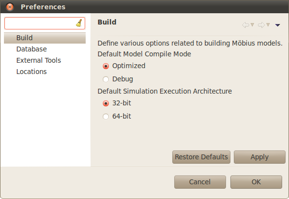
  • Preferences: Launch the preferences window (see <xr id="fig:projman_preferences" />).


<figure id="fig:projman_preferences">

Projman preferences.svg


<xr id="fig:projman_preferences" nolink />: The Möbius Preferences dialog is used to change various preferences about the operation of Möbius.
</figure>


  • Quit: Exit Möbius.

Preferences Dialog

The Preferences dialog (<xr id="fig:projman_preferences" />) provides access to various preferences and settings used during the operation of the Möbius tool. The preferences are broken down into pages listed on the left side of the dialog. Above the pages is a filter text box that you can quickly type a keyword in and the preference pages pertinent to that keyword will be displayed. For example, typing “user” in the filter box will eliminate all the pages except the Database page, because it contains a username field used by the database connection feature.

The Preferences dialog contains the following page:

  • Build: This preference page allows you to define the default compile mode and default simulation execution architecture. Möbius can compile in two modes: normal and optimized. Normal mode incorporates compiler-created debugging symbols into the object files, and uses debug-enabled Möbius AFI libraries when creating the executables, allowing project-generated executables (such as the simulator and state-space generator) to be run through C++ debuggers like gdb. Normal mode also enables Möbius trace output, making it possible to generate files that trace the progress of the model during solution. Normal mode object code takes less time to generate, but is often much larger than optimized code, due to the extra debugging symbols that are included.
Optimized mode enables full compiler optimizations, and disables debug symbols and trace output. Optimized mode should be used when the model is running well, and results need to be produced rapidly.
The results generated should be the same in either mode. The modes allow for the trade-off between extra information needed for debugging and speed of data production.
The default simulation execution architecture mode has two options: 32-bit and 64-bit. For machines running a 32-bit version of their operating system, this setting has no effect as simulations will always be executed in 32-bit mode. However, for machines running a 64-bit operating system, you have the option of building and executing 32-bit or 64-bit simulations. 32-bit simulations will likely run a little faster and take up significantly less memory during execution. However, 64-bit simulations enable access to greater amounts of memory space that may be necessary for large simulations. Simulation results in either mode should be the same.
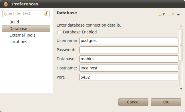
  • Database: The Database settings dialog displays the list settings that are needed to interface Möbius the integrated results database features with the external database server.


<figure id="fig:projman_db">

Projman database.png


<xr id="fig:projman_db" nolink />: The Results Database preference page is used to specify the database access settings.
</figure>


Database Enabled determines if Möbius will connect to the database server using the specified configuration settings.
User Name specifies the name of the database user that Möbius should use when connecting to the database system.
Password specifies the password for the indicated database user.
Database is the name of the database Möbius will create. Multiple databases can be created as needed, simply by changing this name.
Hostname is the name of the machine where the database server is located. Can be a full machine name or “localhost”.
Port is the listening port of the database server. The default port is 5432. Ask your system administrator if the port was changed when the database server was configured.
  • External Tools: The External Tools preference page lists the external tools Möbius uses during its operation. In special cases, you may want to change the tool used to perform a certain operation (for example, the remote shell or archive command). The provided tool must either be in your PATH or the absolute path to the tool should be provided. Some fields are used to specify additional arguments to the external tool whenever it is called.
Compiler: The G++ compiler that Möbius should use.
Compiler Options: Extra compiler options to be used when compiling the Möbius project. This field was originally used to add debugging flags. In current versions, debugging flags are automatically added as part of the normal compilation mode, and this field should typically be blank.
Linker: The linker, ld. Usually set to the path to the standard linker for the system.
Linker Options: Extra linker options to be used when linking Möbius solvers (such as the simulator and state-space generator). For standard use, this field can be left blank.
Make Command: The GNU make tool. The version of make should be 3.7x or later.
Archive Command: The ar tool, the system command used to create C++ library files.
Ranlib Command: The ranlib tool. Ranlib is used during the creation of project libraries.
Remote Shell Command: The command used to gain remote access to other machines on the network. It is not necessary to specify a remote shell command to run Möbius on a single local machine. Typically this command is either rsh or ssh. In either case, system access privileges must be set so that the command can execute without entering a password or pass phrase. More details are available in Appendix section ?? and in the system man pages for rsh and ssh.
Tar Command: The GNU tar command. This command is used to create and restore archive files. NOTE: In the current version of Möbius, tar is used with the “z” option, specifying the archive to be compressed with gzip. Typically gzip is installed in the same directory as tar, but most implementations of tar expect to find gzip in the PATH, and do not expect to have to look for it. If there are error messages when “archive” or “unarchive” commands are run, please see if gzip is found in the system PATH, and update the PATH if necessary.
  • Locations: The locations preference page contains a list of system paths necessary for the operation of Möbius.
Möbius Installation Path: The directory where the Möbius software is installed. This field should update automatically, based on the location of the Möbius executable currently running. Möbius uses this directory to locate the Möbius AFI header files and libraries.
Möbius Projects Directory: The directory containing the desired set of Möbius projects. It is possible to have multiple project directories, and changing this field switches from one to another. Most new users find one project directory is sufficient. The project path should not contain spaces. As a result, the default path on Windows is C:MobiusProject. If multiple people are using Möbius on the same machine, they should all give unique names for their Project directories.


Tools Menu

The Tools menu lists the various utilities available in Möbius. The Data Manager menu item will launch the Möbius Data Manager, which is further described in Section 1 of Utilities.


Help Menu

The Help menu provides various help for the use of Möbius. The About menu item opens the About window. The About window contains information about this version of Möbius, including the vendor and copyright statement.


Console View

The Console View provides a running output of the operations of Möbius. When a project is opened or a model component is saved, this event is logged by the console for your review. The Console View has several icons in the upper right corner to control the behavior of the console and to switch between the available console logs.

The first icon looks like a document with a grey X over it. This icon clears all the text from the current console log. This can be useful for when you want a fresh start to the log.

The next icon has a lock over a scrolling control. This is the scroll lock and will prevent the console from autumatically scrolling down as new text is appended to the console.

The next icon has pin on a window icon. This is the pin console button and will keep the console view from switching to a different console automatically.

Finally, the last icon allows you to switch between the available console logs. The Main console provides general information about the operation of Möbius. The Error console provides detailed error messages when something goes wrong. The Detailed console provides the finest grain of detail messages possible and includes messages from the other two consoles. Of particular interest, when Möbius executes an external command (e.g. make, java, etc.) the command and its arguments are logged in the Detailed console.

The text of a console log can be highlighted for copy/paste operations like you would expect. Also, if you right click on the text, a simple find feature is available to quickly search through the contents of the log.


Project Editor

The Möbius project is the fundamental unit of organization for each system model in Möbius. A complete project will contain the following: one or more models defining the system behavior, a description of what to measure about the system, specification of all model parameters, at least one instantiation of a solver to compute the required measurements, and the results produced by the solver.


Tree View

The model types in the project are classified in the same hierarchy as the components of the Möbius framework (see section 1 of Modeling Background). The model types that may exist in a project are listed below.

  • Atomic models describe the behavior of individual components of the system.
  • Composed models are hierarchical models used to combine atomic and composed models to form the complete model of the system.
  • Reward models define measures of interest about the system.
  • Study models create experiments that specify values for the system parameters in the model.
  • Solvers solve the model using simulation, or prepare the model for numerical solution using state-space generation.
  • Numerical solvers solve the model using a variety of numerical algorithms.

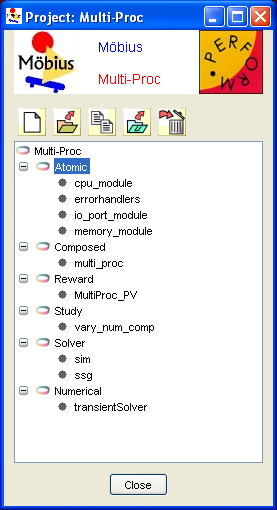
The model types are arranged in a tree, in which the names of the various classifications are the main nodes, and the instances of each classification are the children of the node. The tree view from an example project editor is shown in <xr id="fig:project_main" />.


<figure id="fig:project_main">

Project main.png


<xr id="fig:project_main" nolink />: Tree view in the project editor, with Atomic selected.
</figure>


The order of model types in the tree represents the typical dependency among models in a project. A model of a given type typically depends on models of the type one level above it in the tree. For example, a study model depends on a reward model. When one model depends on another, it is often referred to as the parent, and the model it depends on is referred to as the child.


Project Operations

Several operations are possible in the project editor. You can access the operations via the toolbar or through a pop-up menu activated by right-clicking within the tree view.


New     To create a new model within a project, select the desired category and click on New. A dialog will appear, asking for the type of formalism to create. For example, <xr id="fig:model_creation#1" /> displays the possible types of atomic models that can be created. The dialog also gives the opportunity to name the new model.

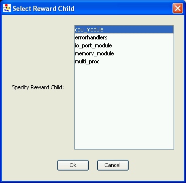
After you click the OK button, the new model editor will open. In the case of the reward, study, solver, and numerical solver models, another pop-up dialog will immediately appear, requesting the name of the child model of the new model, as shown in <xr id="fig:model_creation#2" />.

<figure id="fig:model_creation">

<subfigure>Project atomic.png</subfigure> <subfigure>Project child.png</subfigure>
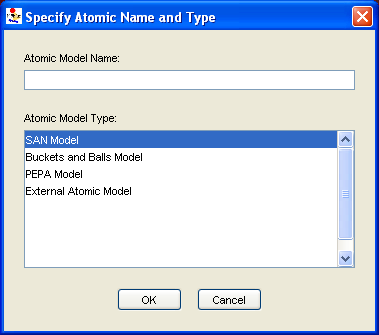
(a) Specify the name and type of newly created models. (b) Specify the newly created model’s child model.
</figure>
<xr id="fig:model_creation" nolink />: Dialogs shown when a new Möbius model is created.


Open     Select a model name from the tree view, and then click Open to open it. Multiple models may be open at the same time.


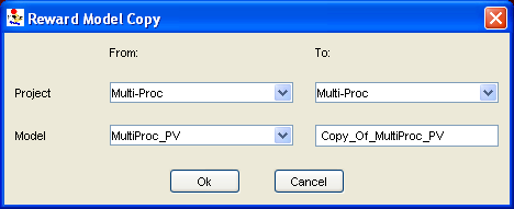
Copy     Select a model name or type from the tree view, and then click Copy to generate a copy of the model. Another dialog opens, allowing you to copy the selected model to another file within this project, or copy it into another project. Also, you can copy models from another project into the current one.


<figure id="fig:project_copy">

Project copy.png


<xr id="fig:project_copy" nolink />: An instance of the copy dialog, which is used to copy models within a project, or from one project to another.
</figure>


Import     Select a model type in the tree view and then click Import to import this type of model from an existing UltraSAN1 project. A dialog will appear, listing all the UltraSAN projects found in the UltraSAN project directory (see Section ?? on how to set the UltraSAN project directory). After you select one of the UltraSAN projects, another dialog will appear listing all possible models in the UltraSAN project of the type selected in Möbius.

1 UltraSAN was the predecessor to Möbius.


Delete     You can delete a model in a Möbius project by selecting the model in the tree view and choosing the Delete menu.


Close     You can close the project editor using the Close button, after all of the model editors of the project have been closed.


Project Directory Structure

Each project is stored in a directory named after the project within the Möbius project directory. It is necessary to understand the basic structure of a project directory, since Möbius stores output files, such as solution results or model documentation, in various locations within the project subtree. Files within the project directory are arranged in the same tree structure as the tree view.

Solution results and other solver outputs are typically written to the model directory corresponding to the solver that generated the results.

All documentation is stored in a subdirectory of the Documentation directory in the top-level directory of the project. The name of this subdirectory is given by the Document Name field in the Document Project dialog. See <xr id="fig:doc_proj" /> for an example.

The project and each model in the project are defined in separate files, which are also named after the project or individual model and have extensions unique to each type of model. The files are XML-based, and under most circumstances should not be edited directly. Doing so can corrupt the Möbius project.


Constraints Checker

When a project, or a submodel within the project, is saved in the Project Editor, the constraints checker is called by the Project Manager to ensure that the model, as saved, doesn’t violate any conditions imposed upon it by solver modules which utilize the model. If the constraints checker detects a violation of a constraint, it produces a pop-up warning informing the user of the problem, prompting them to correct the issue.

For more on specific constraints for individual solvers, see section 4 of Solving Models.


Model Editors

Common Menus

There are several menus that are common to each model editor in Möbius. Instead of describing these features repeatedly, the functionality common to each model editor is discussed in this section.

File

The File menu is common to all editors, and typically contains the following common commands:

  • Save: Store the current model to disk, and then translate the model into the appropriate C++ code and compile the code to form the representative library for this model.
  • Save No Compile: Store the current model to disk, but avoid performing the compilation. It is still necessary to compile the model, either by selecting Save from the File menu, or by compiling within the solver.
  • Close: Close the editor. If there are unsaved changes, a dialog will appear, prompting you to save before closing.
  • Document Model: Create HTML documentation for the current model. The documentation files will be stored in a subdirectory in the Documentation directory within the project’s project directory. The name of the subdirectory will be what you specify in the Document Name field of the dialog box. See <xr id="fig:doc_proj" />.

Edit

Undo

You are allowed to undo most recent operations on the model using the Undo menu. Examples of operations that can be revoked using the undo feature include the movement of graphical components in an editor, the renaming of components, the editing of text, the addition of new components, and the addition of lines. The Undo menu will list the name of the most recently completed operation that can be undone. Undo operations are stored so that multiple operations can be undone.


Edit global variables

The behavior of complex systems being modeled often depends on several parameters. Often these parameters are unknown, or can take on multiple values, depending on the configuration of the system. Möbius provides the option of using global variables instead of pure numerical values to define the different characteristics of elements like state variables and actions. The values of the global variables are then set by experiments in the study model.

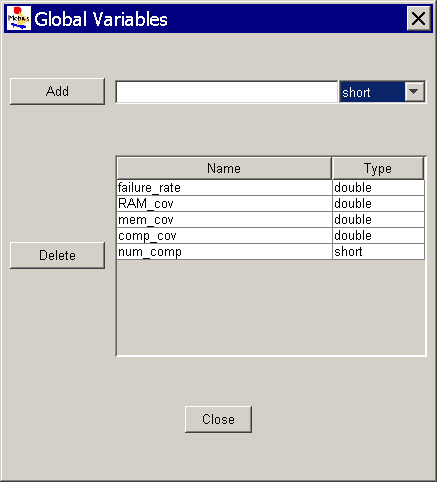
In each atomic or composed model, you can add or delete global variables by clicking on the Edit Global Variables option on the menu editor. A pop-up dialog box, as shown in <xr id="fig:atomic_san_editor_global_variables" />, is used to add, delete, and view global variables. The dialog box can remain open as a reference while you are editing the model.


<figure id="fig:atomic_san_editor_global_variables">

Atomic san editor global variables.png


<xr id="fig:atomic_san_editor_global_variables" nolink />: Global Variables editor.
</figure>


  • The Add button is used to create new global variables. The combo-box on the top-right corner lists the available data types for the global variable. Only the standard data types that C++ directly supports are currently allowed (char, double, int, long, float, and short).
  • The Delete button is used to delete the selected global variables.
  • The Close button is used to hide the Global Variables editor dialog box.


User-defined functions

While building models, you might find it useful to define functions for the model using C++ header files and libraries. These functions are stored in C++ header (.h) or possibly source (.cpp) files that you must create. The files can be placed anywhere, but most often are stored in a new subdirectory in the project. If you are using C++ source files (.cpp), you will also need to place into the same directory a Makefile that will compile the source files into a library. The simplest way to create the Makefile is to copy one from an atomic model in your project and modify it to compile the library. With the current version of Möbius, you must compile the library manually before running a solver. Otherwise, an error message stating the library is missing will appear when the compiler tries to link with the user-defined library in the solver.

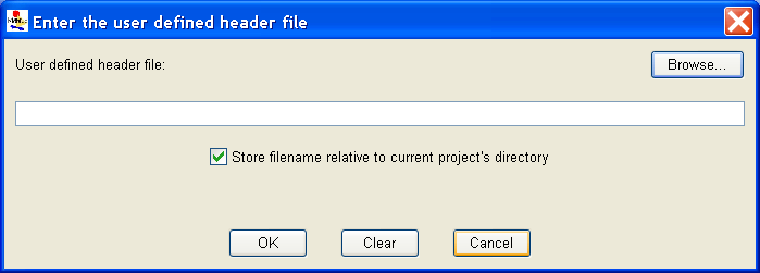
After you have successfully compiled the source code and created the library, you need to let Möbius know the location of the functions. You can do this by opening any model and selecting User-Defined Header under the Edit menu. A dialog box will pop up, asking for the location of your header (see <xr id="fig:atomic_san_editor_user_defined_header" />).


<figure id="fig:atomic_san_editor_user_defined_header">

Atomic san editor user defined header.png


<xr id="fig:atomic_san_editor_user_defined_header" nolink />: User-defined header editor.
</figure>


Enter the path to the C++ header file. There is a check box that instructs Möbius to store the header file path relative to your Möbius project directory. You should check it if your header files are stored in a subdirectory of your project, as it makes it easier to share your project with other users, or relocate it to different systems. If the path entered is incorrect, or the file has not yet been created, Möbius will display an error message.


<figure id="fig:atomic_san_editor_user_defined_library">

Atomic san editor user defined library.png


<xr id="fig:atomic_san_editor_user_defined_library" nolink />: User-defined library editor.
</figure>


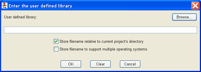
If you are also using a user-defined library, repeat the same operation for the library (see <xr id="fig:atomic_san_editor_user_defined_library" />). This dialog contains the same relative path checkbox found in the User-Defined Header dialog. It also contains another checkbox that makes it possible to support multiple operating system versions of the user-defined library. This feature will only work if the library name contains the name of the current operating system: Solaris, Linux, or Windows. After you check this box, the operating system name is replaced with $ARCH. When Möbius compiles your project on each operating system, $ARCH is replaced with the name of the appropriate operating system.

User-defined functions can be extremely useful if you are trying to make models more modular, or if multiple elements, such as SAN output gates, within the model are performing similar operations. In fact, you can even define functions that would modify the values of elements within the model (for example, a place within a SAN). Here are a few examples in which user-defined functions are helpful:

  • If your model contains complex functions that are repeatedly used or susceptible to change, you can write them in the library and simply call them from the model. For example, to define a comparison between two extended places that are arrays of 2 integers, you can create the following function in the library:
inline int is_lower(int x1, int y1,
int x2, int y2) {
if (x1<x2) return 1;
else if (x1 == x2) {
if (y1 <= y2) return 1;
else return 0;
}
else return 0;
}
The following code shows how to use the function in the model:
short result = is_lower(Place1->x, Place1->y,
Place2->x, Place2->y);
if (result == 1)
...
  • In the same way, you can define enabling conditions for activities using user-defined functions:
inline int activity_enable(int value1,
int value2) {
int ret=0;
if (value1==0 && value2==0)
ret=1;
...
return ret;
}
The enabling function of the corresponding input gate would then call the user-defined function, as follows:
activity_enable(Command1->Mark(),
Command2->Mark(), Group_ID->Mark(),
Component_ID->Mark(),
Component_type->Mark())
  • If you have an extended place in your model with a type that is a large array, matrix, or structure, it is possible to write a user-defined function to initialize the extended place. If you want to create unique experiments that define different initial values for this extended place, you can create a single global variable, and then write the user-defined function so that the extended place is initialized with different values, based on the value of the global variable. Then in the study you only need to adjust one value to change the definition of all fields in the extended place.


Atomic Formalisms

Each model is composed of one or more submodels, also referred to as atomic models. You can create and edit atomic models using different editors like the SAN editor, the PEPA editor, the Buckets and Balls editor, and the Fault Tree editor.


ADVISE

Mobius supports multiple modeling formalisms, including ADversary VIew Security Evaluation (ADVISE). ADVISE allows modelers to create and analyze a specific adversary profile in an executable state-based security model of a system (11LEM02). Using graphical primitives, ADVISE provides a high-level modeling formalism to easily create the adversary profile and the executable state-based security model of the system under consideration.

ADVISE Primitives

ADVISE models consist of five primitive objects: attack steps, accesses, knowledges, skills, and goals. Attack steps represent the actions taken by the adversary. Accesses, knowleges, and skills represent the accesses, knowledge, and skills of the adversary, respectively. Goals represent the goals (or flags) of the adversary.

Attack Step

Attack steps represent the actions taken by the adversary. Attack steps are represented graphically as rectangles. An attack step is fully described by its input, output, and properties. An attack step can have inputs from accesses, knowledges, skills, and goals. It can also have outputs to the same four types of elements (accesses, knowledges, skills, and goals). An attack step also contain four properties: attack cost, attack evaluation time, preconditions, and outcomes.

The attack cost of an attack step represents the relative cost of the attack step with respect to the adversary. For example, if an attack step is difficult or expensive (such as hacking into a locked vault door), then the attack cost will be relatively large. If the attack step is easy or inexpensive (such as opening an unlocked door), then the attack cost will be relatively small. Since an adversary is more likely to take the easiest route to the goal, she will likely choose an attack step with a lower attack cost over one with a higher attack cost.

The attack execution time of an attack step represents the relative time it will take to complete the attack step. For example, if an attack step will take a long time to complete (such as downloading several terabytes of logs), then the attack execution time will be relatively large. If the attack step will not take much time to complete (such as downloading a few kilobytes of a small subset of the logs), then the attack execution time will be relatively small. Since an adversary is more likely to take the quickest route to the goal, she will likely choose an attack step with a shorter attack execution time over one with a longer attack execution time.

The preconditions of an attack step represent the conditions that must take place before the adversary is able to attempt the attack step. The preconditions of an attack step are closely related to the inputs of the attack step since the inputs of the attack step provide the state variables of the model that can be used in the conditional expression. For example, if the attack step requires a certain access and level of skill to attempt, then the inputs of the attack step would be that access and that skill, and the precondition of the attack step would be a conditional expression such as \verb|return (access1 && (skill1 > 0.7)|. As a more concrete example, suppose the attack step is to pick the lock on a safe. The access in this case would be having close proximity to the lock, and the skill would be lock-picking.

The outcomes of an attack step represent the outcomes that occur if the attack step is successfully completed. The outcomes of an attack step are closely related to the outputs of the attack step since the outputs of the attack step provide the state variables of the model that can be modified depending on the resulting outcome. Every attack step has one or more outcomes, each with a probability of occurring. The sum of the probability of each of the outcomes of the attack step is always 1. Each outcome also has an associated detection probability which represents the probability that the adversary will be detected if this outcome occurs. Since an adversary is likely to want to avoid being detected, she will likely choose attack steps with a lower weighted detection probability of its outcomes over an attack step with a higher weighted detection probability of its outcomes.

Access

Accesses represent the relevant accesses the adversary may have (or eventually gain) in the executable state-based security model of the system. Accesses are state variables that store whether or not the adversary has the given access. An access may represent a physical access (such as close proximity to a target or having a key to a relevant door in the model) or a more abstract access (such as administrator privileges in a target machine). Accesses are represented graphically as purple squares.

Knowledge

Knowledges represent the relevant knowledge the adversary may have (or eventually gain) in the executable state-based security model of the system. Knowledges are state variables that store whether or not the adversary has knowledge of the given information. Knowledge may represent a fact such as the adversary knowing a certain password of a target system or the type of encryption that is used between two target nodes. Knowledges are represented graphically as green circles.

Skill

Skills represent the relevant skills the adversary may have (or sometimes may eventually gain) in the executable state-based security model of the system. Skills are state variables that store the extent to which the adversary is skilled in that given area. For example, a certain adversary may have a lock-picking skill of 0.7 which could mean that she is adept at lock-picking, but not yet a master of the skill. Skills are represented graphically as blue triangles.

Goal

Goals (or flags) represent what the adversary is trying to ultimately achieve. Goals are state variables that indicate whether or not the adversary has accomplished the goal yet. Goals can represent achievements such as successfully accessing sensitive information, shutting down a target system, or escaping from a bank with stolen jewels. Goals are represented graphically as gold ovals.

Editor

This section looks into the atomic formalism that represents ADVISE with emphasis on creation, editing, and manipulation of atomic models using the Mobius ADVISE editor.

TODO - Finish this section

Edit

TODO - finish this section

View

TODO - finish this section

Elements

Elements are ADVISE model primitives. The Elements menu includes the following types of elements:

  • Attack step - rectangle
  • Access - purple square
  • Knowledge - green circle
  • Skill - blue triangle
  • Goal - gold oval

TODO - finish this section

SAN

Möbius supports multiple formalisms, including stochastic activity networks (SANs). SANs[1] are stochastic extensions to Petri nets[2]. Using graphical primitives, SANs provide a high-level modeling formalism with which detailed performance, dependability, and performability models can be specified relatively easily.

SAN primitives

SANs consist of four primitive objects: places, activities, input gates, and output gates. Activities represent actions of the modeled system. Places represent the state of the modeled system. Input gates are used to control the “enabling” of activities, and output gates are used to change the state of the system when an activity “completes.”


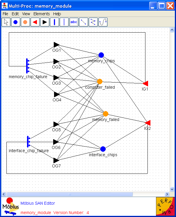
Places     Places represent the state of the modeled system. They are represented graphically as circles. In <xr id="fig:atomic_san_editor" />, memory_chips, interface_chips, memory_failed, and computer_failed are places. Each place contains a certain number of tokens, which represents the marking of the place. The set of all place markings represents the marking of the stochastic activity network. Note that tokens in a place are homogeneous, in that only the number of tokens in a place is known; there is no identification of different kinds of tokens within a place.


<figure id="fig:atomic_san_editor">

Atomic san editor.png


<xr id="fig:atomic_san_editor" nolink />: Möbius SAN Editor.
</figure>


The meaning of the marking of a place is arbitrary. For example, the number of tokens in a place could represent a number of objects, such as a number of tasks awaiting service. Also, the number of tokens in a place could represent an object of a certain type, such as a task with a certain priority level. This dual nature of a place marking provides a great deal of flexibility in modeling the dynamics of a system.


Activities     Activities represent actions in the modeled system that take some specified amount of time to complete. They are of two types: timed and instantaneous. Timed activities have durations that impact the performance of the modeled system, such as a packet transmission time or the time associated with a retransmission timer. Timed activities are represented graphically as thick vertical lines. In <xr id="fig:atomic_san_editor" />, memory_chip_failure and interface_chip_failure are timed activities. Each timed activity has an activity time distribution function associated with its duration. Activity time distribution functions can be generally distributed random variables. Each distribution can depend on the marking of the network. For example, one distribution parameter could be a constant multiplied by the marking of a certain place. Instantaneous activities represent actions that complete immediately when enabled in the system. They are represented graphically as thin vertical lines. No instantaneous activities are represented in <xr id="fig:atomic_san_editor" />. Case probabilities, represented graphically as circles on the right side of an activity, model uncertainty associated with the completion of an activity. Each case stands for a possible outcome, such as a routing choice in a network, or a failure mode in a faulty system. In <xr id="fig:atomic_san_editor" />, activity interface_chip_failure has three cases. Each activity has a probability distribution, called the case distribution, associated with its cases. This distribution can depend on the marking of the network at the moment of completion of an activity. If no circles are shown on an activity, one case is assumed with a probability of one.

An activity is enabled when the predictes of all input gates connected to the activity are true, and all places connected to incoming arcs contain tokens, i.e. have non zero markings. Once enabled, the activity samples its delay distribution function to determine the time delay before the activity fires. When the activity fires it updates the state of the model by subtracting tokens from places connected by incoming arcs, adding tokens to places connected by outgoing arcs, and executing the functions in input and output gates. The specific order that the state updates occur is: input gates, input arcs, output gates, and finally output arcs.

Please be aware that the order in which state updates occur in Möbius differs from UltraSAN. Gates are executed before arcs in Möbius, but the opposite was true in UltraSAN. Also, if there are multiple instances of the same item, for instance multiple input gates, the order of application of the gates is not specified. Models must be constructed so that the gate functions are execution order independent any time there are multiple instances of the same type of gates connected to an activity.

Also associated with each activity is a reactivation function. This function gives marking dependent conditions under which an activity is reactivated. Reactivation of an activated activity means that the activity is aborted and that a new activity time is immediately obtained from the activity time distribution. The reactivation function consists of an activation predicate and a reactivation predicate. An activity will be reactivated at the moment of a marking change if (1) the reactivation predicate holds for the new marking, (2) the activity remains enabled, and (3) the activation predicate holds for the marking in which the activity was originally activated.


Input gates     Input gates control the enabling of activities and define the marking changes that will occur when an activity completes. They are represented graphically as triangles. In <xr id="fig:atomic_san_editor" />, IG1 and IG2 are input gates. On the other side of the triangle is a set of arcs to the places upon which the gate depends, also called input places. Each input gate is defined with an enabling predicate and a function. The enabling predicate is a Boolean function that controls whether the connected activity is enabled. It can be any function of the markings of the input places. The input gate function defines the marking changes that occur when the activity completes.

If a place is directly connected to an activity with an arc, it is equivalent to an input gate with a predicate that enables the activity whenever the place has more than zero tokens along with a function that decrements the marking of the place whenever the activity fires.


Output gates     Like input gates, output gates define the marking changes that will occur when activities complete. The only difference is that an output gate is associated with a single case. An output gate is represented graphically as a triangle with its flat side connected to an activity or a case. In <xr id="fig:atomic_san_editor" />, OG1, OG2,..., OG6, and OG7 are output gates. On the other side of the triangle is a set of arcs to the places affected by the marking changes. An output gate is defined only with a function. The function defines the marking changes that occur when the activity completes. There is also a default scenario for output gates. If an activity is directly connected to a place, it is equivalent to an activation in which an output gate has a function that increments the marking of the place whenever the activity is fired.

More information on SANs can be found in [1]. The next few sections describe the various features available in the SAN editor to develop a SAN model.

Editor

This section looks into the atomic formalism that represents stochastic activity networks with emphasis on creation, editing, and manipulation of atomic models using the Möbius SAN editor. Refer to Section 2 for details on how to create and open a SAN model.

The names of the selected project and subnet appear in the top left corner (see <xr id="fig:atomic_san_editor" />). The large gridded area in the center is the drawing area . In the case of a new model, this gridded area is blank. Like most applications, the editor lists the menu horizontally at the top of the application’s current active window. If you click on a menu item, it drops a tool panel containing several options. The menu items and tool panel options are used to create and draw in the SAN formalism, as discussed below.

As discussed in Section 3.1, many menus are common to all model editors within Möbius. Please see Section 3.1 for detailed descriptions of the common editor functions. The following paragraphs will discuss the functionality that is unique to the SAN editor.

Edit

Type definitions

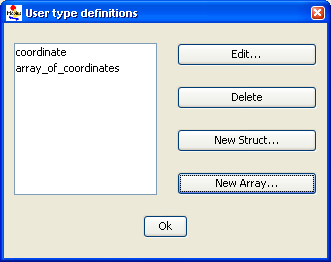
The SAN formalism supports a special element called extended place that allows the model to handle the representation of structures and arrays of primitive data-types. Clicking on Type Editor opens the dialog box shown in <xr id="fig:atomic_san_editor_user_type_definition" />. In this dialog box, you can create new structures and arrays that can be associated with extended places.


<figure id="fig:atomic_san_editor_user_type_definition">

Atomic san editor user type definition.png


<xr id="fig:atomic_san_editor_user_type_definition" nolink />: SAN user-type definition editor.
</figure>


  • Use the Edit button to edit any currently defined user-defined types. The GUI can automatically tell if the user is editing an array (see <xr id="fig:atomic_san_editor_user_type_definition_array" />) or structure (see <xr id="fig:atomic_san_editor_user_type_definition_structure" />) and appropriately open the required editor. You are expected to click on the available list of user-defined types to edit them. The editor allows you to change the name of any user-defined type, even if the user-defined type is declared as a field in another user-defined type or associated with an extended place. The interface takes care of updating all the changes.
  • Use the Delete button to delete the selected user-defined type that is not being used by any other user-defined type and is not associated with any extended place. If you attempt to delete a type that is in use, an error dialog box pops up. A successful delete removes the user-defined type from the current list.
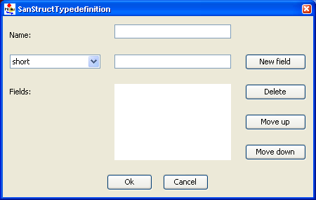
  • Use the New Struct button to pop up a new dialog box that allows you to create a new structure-type definition. The pop-up dialog box layout is depicted in <xr id="fig:atomic_san_editor_user_type_definition_structure" />.


<figure id="fig:atomic_san_editor_user_type_definition_structure">

Atomic san editor user type definition struct.png


<xr id="fig:atomic_san_editor_user_type_definition_structure" nolink />: SAN struct-type definition editor.
</figure>


– Use the Name text box to define a name for the structure.
– The Fields list shows the fields you declared in the current structure.
– The New field button adds a new field to the structure. The combo-box on the left lets you choose the type of the field from a list of the standard data types and user-defined data types. Recursive definitions or pointers are not allowed.
– The Delete button deletes the selected field.
– The Move up button moves the selected field up by one position.
– The Move down button moves the selected field down by one position.
– The OK button accepts all changes made and hides this dialog box, bringing the User-type definitions editor to the front. An error message pops up you try to create a structure with no fields or a structure that has no name or a non-unique name.
– The Cancel button discards all changes, hides this dialog box and returns you to the User-type definitions editor.
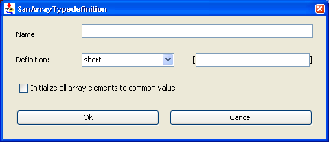
  • The New Array button pops up a new dialog box that allows you to create a new array-type definition. The pop-up dialog box layout is depicted in <xr id="fig:atomic_san_editor_user_type_definition_array" />.


<figure id="fig:atomic_san_editor_user_type_definition_array">

Atomic san editor user type definition array.png


<xr id="fig:atomic_san_editor_user_type_definition_array" nolink />: SAN array-type definition editor.
</figure>


– The Name text box allows you to define a name for the array.
– The Definition combo-box allows you to select the data type for the array. The choices include primitive data types or user-defined types. You are also expected to declare the size of the array. The elements of the array are generically labeled as index.
– The Initialize all array elements to common value checkbox makes it easier to manage large arrays. If it is known when the array type is defined that all elements in the array should be initialized to the same value, 0 for instance, clicking this box will avoid the need to initialize each element separately. This option is critical when defining very large arrays because it saves a significant amount of memory within the Möbius editor process.
– The OK button accepts all changes made, hides this dialog box, and returns you to the User-type definition editor. An error message will pop up if you try to create an array with an invalid size (i.e., a non-numeric, zero, or negative size) or an array that has no name or a non-unique name.
– The Cancel button discards all changes, hides this dialog box, and brings you back to the User-type definition editor.
  • The OK button hides the User type definitions dialog box and brings you back to the SAN editor.

View

Increase size and Decrease size

Click on menu item Increase Size to increase the size of the drawing area. Click on Decrease Size to decrease the size until the scroll bar disappears or becomes equal to area on which the model elements are spread. You can increase the size of the drawing area, scroll down to the extra space created, and add new components to the model, if necessary.


Zoom in and Zoom out

Each time you click on the menu item Zoom In, the GUI enlarges the drawing area by a fixed percentage. The interface takes care of adding scroll bars if necessary so that the entire model can be viewed. To keep the model in focus, be careful not to multiple-click on this option. Zoom Out decreases the size of the model until the scroll bars disappear.


Grid setting

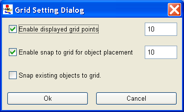
Click on the menu item Grid Setting to open a dialog box as shown in <xr id="fig:atomic_san_editor_grid_setting" />. Here, you can define the X and Y coordinate size of the grid in pixels. Note that if you set the grid to 1 pixel size, it will take an extremely long time to render the model. You can adjust the grid according to your comfort level. There are a few checkboxes on the Grid Setting dialog box. They are Enable display grid points, Enable snap to grid for object placement, and Snap existing objects to grid. Each checkbox is self-explanatory. Use the OK button to accept the changes or the Cancel button to discard the changes. Either way the dialog box will close so that you are returned to the SAN Editor.


<figure id="fig:atomic_san_editor_grid_setting">

Atomic san editor grid setting.png


<xr id="fig:atomic_san_editor_grid_setting" nolink />: SAN user Grid Setting Dialog editor.
</figure>


Elements

Elements are SAN model primitives. The Elements menu includes the following types of elements:

  • Place, which will be represented by a blue circle.
  • Extended Place, which will be represented by an orange circle.
  • Input Gate, which will be represented by a triangle with its tip pointing to the left.
  • Output Gate, which will be represented by a triangle with its tip pointing to the right.
  • Instantaneous Activity, which will be represented by a solid vertical bar. If the activity has multiple cases, they appear as small circles on the right side of the vertical bar.
  • Timed Activity, which will be represented by a hollow vertical bar. It has small circles on its right side if it has multiple cases.

You can also select a SAN model element by clicking the left button on the required component while the cursor is on the menu item Elements. SAN elements can also be accessed via icons below the menu. To place one of those components, click on it, move it to the desired location, and place it by clicking the left mouse button. A dialog box will appear asking you to specify various attributes relevant to the element type. The name must be unique across the current atomic model. The name also must follow the C++ variable naming convention. The rest of this section discusses various parameters of each model element.


Place

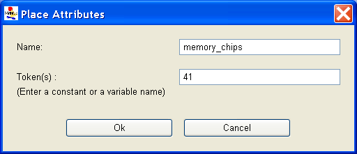
When you create or edit a place (by right-clicking on the place and clicking on Edit in the pop-up window), a dialog box similar to the one shown in <xr id="fig:atomic_san_editor_place_attribute" /> appears.


<figure id="fig:atomic_san_editor_place_attribute">

Atomic san editor place attributes.png


<xr id="fig:atomic_san_editor_place_attribute" nolink />: Place Attributes dialog box.
</figure>


  • The Name text box allows you to modify the name, provided that the new name is unique in the current model.
  • The Token(s) text box allows you to edit or modify the initial marking. The value should be a non-negative short integer, which implies that place markings can only be non-negative integers less than or equal to 32,767. However, the initial marking may be defined as a scalar value, or as a global variable. The following points about global initial marking must be noted:
– global variables for places must be of type short.
– global variables for initial markings should not be arithmetic expressions, or functions of other initial global markings.
  • The OK button accepts the changes and returns you to the SAN Editor. It pops up an error message if there is a problem in validating the tokens text box.
  • The Cancel button discards the changes and brings you back to the SAN Editor.


Extended place

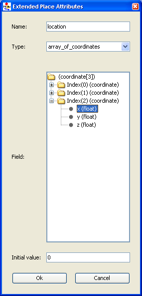
When you create or edit an extended place (by right-clicking on an extended place and clicking on Edit in the pop-up window), a dialog box similar to that shown in <xr id="fig:atomic_san_editor_extended_place_attribute" /> appears.


<figure id="fig:atomic_san_editor_extended_place_attribute">

Atomic san editor extendedplace attributes.png


<xr id="fig:atomic_san_editor_extended_place_attribute" nolink />: Extended Place Attributes dialog box.
</figure>


  • The Name text box allows you to modify the name provided that the new name is unique in the current model.
  • The Initial value tree represents the current values associated with the structure or array of the extended place. Only the leaf nodes can be initialized to a particular initial value. Clicking on intermediate nodes hides the visible text box. Each time you click on a new leaf node, the GUI evaluates the current initial value for validity, displaying error messages if necessary.
  • The text box allows you to edit/modify the initial marking(s) of the selected leaf nodes of the structure or an array. However, the initial marking may be defined as a scalar value, or as a global variable. The following points about global initial marking should be noted:
– global variables for extended places must be of the same type as the corresponding leaf field.
– global variables for initial markings should not be arithmetic expressions, or functions of other initial global markings. Note that the current SAN editor only allows global variables of primitive data types.
  • The Type combo-box allows you to associate a user-defined type with an extended place. Whenever you change the user-defined type, its values are initialized to 0. The Tree is re-drawn with the new structure or array.
  • The OK button accepts the changes and brings you back to the SAN editor. It pops up an error message if there is a problem in validating the tokens text box.
  • The Cancel button discards the changes and returns you to the SAN editor.


Input gate

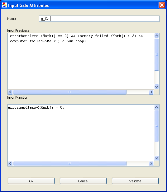
When you create or edit an input gate (by right-clicking on an input gate and clicking on Edit in the pop-up window), a dialog box similar to the one shown in <xr id="fig:atomic_san_editor_input_gate" /> is displayed.


<figure id="fig:atomic_san_editor_input_gate">

Atomic san editor input gates.png


<xr id="fig:atomic_san_editor_input_gate" nolink />: SAN Input Gate Attributes editor.
</figure>


When defining an input gate, be aware of the following points:

  • You must specify a predicate and a function.
  • Input predicates must return a Boolean value. They may be an expression or a sequence of C statements.
  • Input functions are sequences of C++ statements.
  • No return statements are needed in function specifications, since their action is to change the marking of a SAN, not to return a value.
  • If no action is desired in a function (the identity function), this is specified by a lone semicolon.
  • Global variables, places, and extended places may be used in defining input gates.


Special note on programming with extended places     While defining the function of an input gate or output gate, you can use extended places. You can access the fields of a structure using standard C++ dereferencing of pointers. Consider a scenario in which an extended place “ep” is associated with a user-defined structure called “coordinates” as shown in <xr id="fig:atomic_san_editor_user_type_definition_structure" />, with three fields “x,” “y,” and “id” of types short, short, and char. To access field “x” in any function of a gate, use ep->x->Mark(). In another scenario, extended place “ep” is associated with a user-defined array called “ten_type” that is an array of ten elements of type short. Each of these elements of “ep” can be accessed using the method ep->Index(i)->Mark() where “i” can be a previously defined variable. Remember, it is possible to program user-defined variables with arrays and structures using a similar technique by applying the above-discussed rules recursively.


Output gate

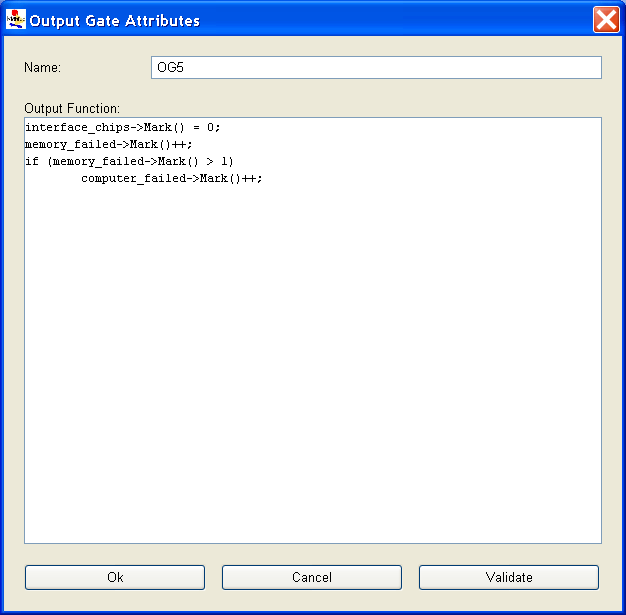
When you create or edit an output gate (by right-clicking on an output gate and clicking on Edit in the pop-up window), a dialog box similar to that shown in <xr id="fig:atomic_san_editor_output_gate" /> appears.


<figure id="fig:atomic_san_editor_output_gate">

Atomic san editor output gates.png


<xr id="fig:atomic_san_editor_output_gate" nolink />: SAN Output Gate Attributes editor.
</figure>


Be aware of the following points regarding definition of output gates:

  • Only one function is needed.
  • Output functions are sequences of C++ statements.
  • No return statements are needed in function specifications, since their action is to change the marking of the SAN, not to return a value.
  • If no action is desired in a function (the identity function), this is specified by a lone semicolon.
  • You may use global variables, places and extended places while defining output gates. Refer to comments in the previous section on programming with extended places.


Activity

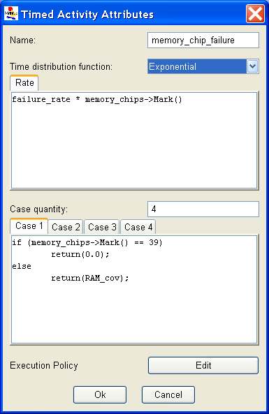
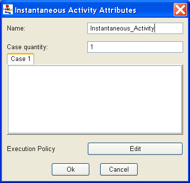
The SAN formalism models activities with two types of elements: timed activity and instantaneous activity. Right-clicking on an activity element pops up a menu that has an option to edit the activity. A dialog box similar to those shown in <xr id="fig:atomic_san_editor_time_activity" /> and <xr id="fig:atomic_san_editor_instantaneous_activity" /> may appear depending on the type of activity created.


<figure id="fig:atomic_san_editor_time_activity">

Atomic san editor time activity.png


<xr id="fig:atomic_san_editor_time_activity" nolink />: Timed Activity Attributes editor.
</figure>


<figure id="fig:atomic_san_editor_instantaneous_activity">

Atomic san editor instantaneous activity.png


<xr id="fig:atomic_san_editor_instantaneous_activity" nolink />: Instantaneous Activity Attributes editor.
</figure>


The steps involved in defining the activities of the model element timed activity are as follows:

  • Specify an activity distribution function by clicking the selector next to the desired distribution in the box titled Time distribution function. For analytic solutions, only exponential and deterministic distributions may be selected.
  • Next, enter the parameters for the chosen distribution in the box below the combo-box. The headings on the box change depending on the distribution chosen. For the exponential distribution, only the rate, which is the reciprocal of the mean, is required. Section 1.2.5 of Modeling Background describes the distribution functions for timed activities in Möbius together with their parameters. The parameters can be expressions (double-precision values), global variables of type double, or series of statements. If statements are used, you must provide a return statement with a double-precision value equaling the parameter.

If more than one case is specified, an additional sub-window is present for specifying the case probabilities. Only one case is visible at a time, but you can step through the remaining cases by clicking on the tab of the case number.

Some points to be noted are:

  • The first case probability corresponds to the top circle on the activity.
  • Case probabilities can be expressions (double-precision values between zero and one), or series of statements (as in <xr id="fig:atomic_san_editor_time_activity" />). If a case probability is a series of statements, then you must provide a return statement with the desired value.
  • Case probabilities may depend on the markings of places, but need not be connected to those places.
  • Case probabilities can be functions of global variables, place markings, and extended place markings.
  • Möbius automatically normalizes the case probabilities.


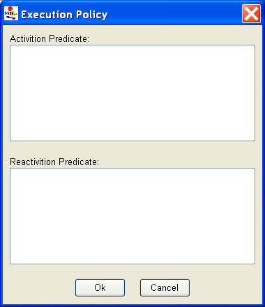
Execution policy

The execution policy editor is an advanced concept that only applies to simulation-based solutions and can be safely ignored for many models. Reactivation is disabled by default, and often this behavior is sufficient. Reactivation is disabled when both the activation and reactivation predicates are undefined, or have a defined value that is false. Refer to Section 1.2.4 of Modeling Background for more information on execution policy.

Reactivation is used to change the behavior of the activity during simulation. When reaction is disabled, the distribution function of an activity is sampled only during the state where the activity is first enabled (i.e., when all input gates associated with the activity are enabled. In more advanced scenarios, the behavior of the model might required that the activity might be activated again (re-activated) so that its distribution is resampled based on the new state of the model. In such cases, the user can set predicates in the Activation Predicate and Reactivation Predicate boxes. In each state where the activation predicate is true, the simulator will check the given activity to determine if it should be reactivated. If the reactivation predicate is also true in the current state, the activity will be reactivated, meaning a new delay will be sampled from the distribution function, and the activity will be scheduled to fire after “delay” units of time from the current simulation time. The reactivation predicate affects the activity only if the activity is already enabled (Modeling_Background#fig:action <xr id="fig:action" /> (d) of Modeling Background). Enabling of the activation predicate could possibly cause scenario (c) in Figure 3 of Modeling Background <xr id="fig:action" />.

<xr id="fig:atomic_san_editor_execution_policy" /> depicts the dialog box that appears with the Execution Policy editor.


<figure id="fig:atomic_san_editor_execution_policy">

Atomic san editor execution policy.png


<xr id="fig:atomic_san_editor_execution_policy" nolink />: Execution Policy editor.
</figure>


Arcs and lines

In SAN models, three arc tools are used for drawing: straight, spline, and connected lines. You use them by selecting one of the arc tools with the left mouse button. Move the mouse to the desired point of origin of the line, and click the left button. Move the mouse to the desired locations of all intermediate points one by one, clicking the left mouse button (for splines and connected lines) to set down each point. When the destination is reached, click the left button. If one of the end points of the line cannot be identified as an appropriate object, an error message appears. You can avoid that by placing the end points clearly within the boundaries of the desired endpoint objects. Lines may overlap objects or other lines. You can cancel an arc you are drawing by right-clicking the mouse.

Note that lines are directed and thus may be drawn only between certain objects in a certain order as listed below:

  • from a place to an activity
  • from a place or an extended place to an input gate
  • from an activity to a place
  • from an activity to an output gate
  • from an input gate to an activity
  • from an output gate to a place or an extended place

Any other combination or order causes an error message to appear. An arrow is automatically placed at the head of the arc when you connect a place directly to an activity, or an activity directly to a place.

You do not need to draw arcs between input/output gates and the places/extended places. Doing so aids in keeping track of interaction between these elements. However, the arc can be left out if including it would clutter the model.


Text boxes

Text boxes have been provided to allow programmers to write comments about the model in the drawing area. They do not affect the behavior of the model in any way. Text boxes are meant to be useful tools for documenting parts of the model. To enter a text box within the drawing area, first select the Text Box element from the Element menu. Next, place the cursor (which appears as an arrow) by the object in the drawing area by which the text is to be entered and click on the left button. Write the text to be displayed in the pop-up dialog that appears. You can edit the text by right-clicking on the text box and selecting Edit.

Useful techniques

This section outlines tricks and techniques that advanced users might find helpful when constructing their models.


Simulation time

If you would like for components in the model to access the current simulation clock, its value can be accessed from C++ code within a given SAN component using this static class member:
BaseModelClass::LastActionTime. The definition of BaseModelClass can be found in <Mobius Installation Root>
/Cpp/BaseClasses/BaseModelClass.h
.

The value is usable only when the model is solved via simulation; thus, models that depend on this value cannot be solved using the state-space-based numerical solution techniques available in Möbius.


Direct use of distribution functions

Advanced users have asked for the ability to generate random numbers using the same set of distribution functions that are used by Möbius. They can do so within the C++ code of SAN model components by adding code similar to this to the component definition:

static UserDistributions dist(0, 31415);
double delay=dist.Exponential(.5);

The first parameter passed to the UserDistributions constructor specifies the type of random number generator to use with this UserDistributions object (0 is Lagged Fibonacci; 1 is Tausworthe). The second parameter sets the initial seed of the random number generator (31415 is known to provide a relatively long period).

For a complete list of the available distribution functions and their arguments, please refer to this Möbius AFI header file:
     <Mobius Installation Root>
/Cpp/simulator/Distributions.h
.

Buckets and Balls

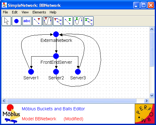
Another formalism supported by Möbius is that of Buckets and Balls. Buckets and Balls provides a method for modeling simple systems for which a SAN might not be necessary. While it lacks the capabilities of a SAN, it is often more appropriate for those systems and subsystems that do not require the complexity offered by other formalisms.

Buckets and Balls primitives

Buckets and Balls consists of two primitive objects: buckets and transitions. Buckets represent the current state of the system, and transitions represent activities and are used to change the state of the system.


Buckets     Buckets are used to represent the state of the model. In the editor, they are represented graphically as circles. Each bucket can contain a certain number of balls, which are used to indicate system state. All balls in a given bucket are assumed to be homogeneous. Thus only the current number of balls in a given bucket is known; there is no method for distinguishing one ball from another in a given bucket.

As with SAN models, the meaning of the state of a given bucket is arbitrary. It could just as easily be jobs in a queue, failures propagating through a system, or an inventory model, for example.


Transitions     Transitions represent events that can change the state of the system. There are two types of transitions available for the Buckets and Balls formalisms: timed and instantaneous. Timed transitions are fired according to their time distribution functions. Transition time distribution functions can be any generally distributed random variables and can be dependent on both variables and the current state of the system. All transitions are represented graphically as lines with arrows indicating the direction of the transition. Timed transitions fire at their generated event times. Instantaneous transitions complete immediately when enabled by the system. It is important to note that only one instantaneous transition may fire from a given bucket at any one time. As there are often many transitions from a single bucket, it is necessary to determine an order for the firings. This order is determined based on the transitions’ weights and ranks. For each rank, all transitions are considered and identified as valid or invalid; the order in which the valid transitions are fired is determined probabilistically. If no valid transitions exist of a given rank, those of a lower rank are considered in the same manner. After a timed transition fires, instantaneous transitions will continue to fire until no more are valid, at which point the model will activate the next timed transition on the event list and proceed as before.

Editor

This section covers the atomic formalism of Buckets and Balls including the creation, editing, and manipulation of atomic models using the Möbius Buckets and Balls editor. Refer to Section 2 for details on how to create and open a Buckets and Balls model.


<figure id="fig:atomic_bucketsballs_editor">

Atomic bucketsballs editor.png


<xr id="fig:atomic_bucketsballs_editor" nolink />: Buckets and Balls editor.
</figure>


As in the SAN model editor, the name of the selected project appears in the top left corner along with the name of the current atomic model. The grid in the center of the interface is the drawing area and is initially blank for a newly created model. Drop-down menus are listed horizontally at the top of the active window and contain tools and options for working with the Buckets and Balls formalism. Some of the menus are common to all model editors in Möbius; please see Section 3.1 for a detailed description of these common editor functions.

Edit

The Buckets and Balls formalism has no unique features in the Edit menu; all functions are the same as those described in Section 3.1.

View

The view menu for the Buckets and Balls formalism is identical to that found in the SAN formalism. Please refer to Section 4.2.4 for more information on the options provided in this menu.

Elements

Elements are Buckets and Balls model primitives. The Elements menu includes the following types of elements:

  • Bucket, which will be represented by a blue circle.
  • Timed Transition, which will be represented by a black line with an attached arrow indicating the direction of the transition.
  • Instantaneous Transition, which will also be represented by a black line with an attached arrow indicating the direction of the transition.

Buckets and Balls model elements can be selected either through the menu item Elements or via the icons below the menu. To place one of these components, simply click on it, move it to the desired location, and place it by clicking the left mouse button. A dialog box will then appear, requesting that you specify the attributes related to the element’s type. As with the SAN model formalism, all names must be unique across the atomic model. All names must also conform to C++ variable naming conventions. For more information on placing transitions, please see the subsection on arcs and lines below.


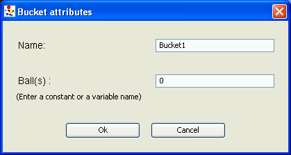
Buckets

When you are creating or editing a bucket (which you do by right-clicking on the bucket and selecting Edit in the pop-up window), a dialog box similar to the one illustrated in <xr id="fig:atomic_bucketsballs_editor_bucket_attribute" /> is shown.


<figure id="fig:atomic_bucketsballs_editor_bucket_attribute">

Atomic bucketsballs editor bucket attribute.png


<xr id="fig:atomic_bucketsballs_editor_bucket_attribute" nolink />: Buckets and Balls bucket editor.
</figure>


  • The Name text box allows you to modify the name of the bucket, provided the new name is still unique in the current model.
  • The Ball(s) section of the dialog contains a radio button to allow you to select either a constant or variable to represent the number of balls in this bucket.
– If Constant is selected, you must enter a non-negative short integer, that is any number greater than or equal to zero and less than or equal to 32,767.
– If Variable is selected, you must enter a global variable of the type short.
  • The OK button accepts any changes you may have made and returns you to the Buckets and Balls Editor. If there are any problems with changes you have made, an error message will appear, indicating the error and asking you to rectify it.
  • The Cancel button discards all changes and returns you to the Buckets and Balls Editor.


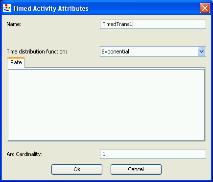
Timed transition

When you are creating or editing a timed transition (which you do by right-clicking on a timed transition and clicking on Edit in the pop-up window), a dialog box similar to that illustrated in <xr id="fig:atomic_bucketsballs_editor_bucket_timedtrans_attributes" /> is shown.


<figure id="fig:atomic_bucketsballs_editor_bucket_timedtrans_attributes">

Atomic bucketsballs editor bucket timedtrans attributes.png


<xr id="fig:atomic_bucketsballs_editor_bucket_timedtrans_attributes" nolink />: Buckets and Balls timed transition editor.
</figure>


  • The Name text box allows you to modify the name, provided that the new name is unique in the current model.
  • The Arc Cardinality text box allows you to set the number of balls transferred by the timed transition when it fires. Note: the transition will not occur for a given bucket if the number of balls in the bucket is less than the number set in this text box.
  • The Time distribution function section of the dialog contains a pull-down menu of the general distributions available for a timed transition and a Parameters button that opens a dialog to allow you to parameterize the selected distribution. Section 1.2.5 of Modeling Background describes the distribution functions for timed activities in Möbius along with their parameters. The parameters can be expressions, global variables of type double, or a series of statements. As with the SAN atomic models, if a series of statements is used, you must provide a return statement with a double-precision value for the parameter.
  • The OK button accepts any changes you may have made and returns you to the Buckets and Balls Editor. If there are any problems with changes you have made, an error message will appear, indicating the error and asking you to rectify it.
  • The Cancel button discards all changes and returns you to the Buckets and Balls Editor.


Instantaneous transition

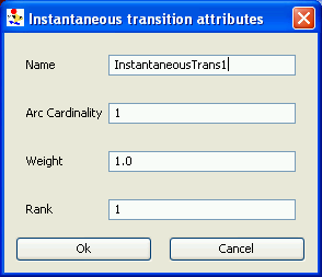
When you are creating or editing an instantaneous transition (which you do by right-clicking on an instantaneous transition and clicking on Edit in the pop-up window), a dialog box similar to that illustrated in <xr id="fig:atomic_bucketsballs_editor_bucket_insttrans_attributes" /> is shown.


<figure id="fig:atomic_bucketsballs_editor_bucket_insttrans_attributes">

Atomic bucketsballs editor bucket insttrans attributes.png


<xr id="fig:atomic_bucketsballs_editor_bucket_insttrans_attributes" nolink />: Buckets and Balls instantaneous transition editor.
</figure>


  • The Name text box allows you to modify the name, provided that the new name is unique in the current model.
  • The Arc Cardinality text box allows you to set the number of balls transferred by the timed transition when it fires. Note: the transition will not occur if the number of balls is less than the number listed in the text box.
  • The Weight text box allows you to set a probabilistic weight for the transition (as only one transition may be selected out of each bucket), these weights will be normalized for all transitions of the specified rank for a given bucket. The weight may be expressed as a variable or as a double-precision value.
  • The Rank text box allows you to set the rank of this transition, indicating its priority with respect to the bucket of origin. Higher-valued ranks will be selected first unless they cannot fire, in which case lower-valued ranks will be selected. Rank may be expressed as a variable or a constant.
  • The OK button accepts any changes you may have made and returns you to the Buckets and Balls Editor. If there are any problems with changes you have made, an error message will appear indicating the error and asking you to rectify it.
  • The Cancel button discards all changes and returns you to the Buckets and Balls Editor.


Arcs and lines

In Buckets and Balls models, as in SAN models, there are three arc drawing tools at your disposal: straight, spline, and connected lines. In a Buckets and Balls model, these arcs define the timed and instantaneous transitions. In order to draw an arc, you simply select one of the arc tools with the left mouse button. Move the mouse to a bucket and click with the left mouse button to set the origin bucket for the transition. If you are drawing a spline or connected line, click the left mouse button in the drawing area to set control points. Finally, click the left mouse button on the destination bucket to create the transition arc. If at any point you wish to cancel the arc, right-click on the drawing area. Arcs may overlap other objects and other arcs. All arcs and lines are directed, and therefore must have both of their endpoints anchored at buckets.


Text boxes

As in the SAN model editor, text boxes have been provided to allow programmers to write comments about different aspects of their models within the drawing area. These comments have no effect whatsoever on the functioning of the model, although they may help another programmer understand the model. For more information on creating and editing text boxes, please see “Text boxes” in Section 4.2.5.

PEPA

Möbius also supports PEPA as a modeling formalism. PEPA, unlike the SAN or the Buckets and Balls formalisms, is a process algebra. Instead of creating a PEPA atomic model in a graphical editor, the model is created using an editor provided in Möbius in a form that resembles a formal language. Möbius extends the basic PEPA language to include process parameters, guards, and value passing. This extension is known as the PEPAk language.

The PEPAk language

This section covers the basic building blocks of the PEPAk language including process variables, formal parameters, guards, choices, prefixes, hide, and cooperation.

  • Process Variable: In the PEPAk language, processes are represented using process variables. A process variable is defined by assigning an equation to a symbolic name using the assignment operator “=”. For example, the following defines the process variable P:
P[a] =
[a > 5] => (\alpha,x).P[a-1]
+ [(a > 0) && (a < 5)] => (\beta,x).P[a-1];


  • Formal Parameters: The PEPAk language extends PEPA to include the possibility of formal parameters for process variables. In the example above the process variable P takes a single parameter, a. More parameters may be specified by a comma delimited list as follows: P[a,b].
  • Guards: The introduction of guards to the PEPAk language allows the selective enabling and disabling of a process expression based on the guard conditions. A process expression is enabled if its guard evaluates to true, and disabled if its guard evaluates to false. Guards are represented by boolean expressions enclosed in square brackets before a process expression, and may contain references to formal parameters. In the above example, the two process expressions are guarded by conditions, [a > 5], and [(a > 0) && (a < 5)]. Thus the first process expression is enabled only if the parameter a is greater than five, and the second process expression is enabled only if the parameter a is greater than zero and less than five. The guard operator “=>” assigns a process expression to a given guard expression.
  • Choice: The choice operator “+” is used to allow a process to behave in different ways under different circumstances as defined by a process expression. The first enabled process expression to complete is selected and the remainder of the expressions are discarded. In the above example we see a choice between two guarded process expressions.
  • Prefix: The simplest way to describe the behavior of a process is to add a prefix to the preferences to the process variable. Prefixes are denoted using the form (\alpha, x).P, where \alpha is some action which has a duration that is exponentially distributed with rate x. After the action has completed, it then behaves according to the referenced process variable. In the case of a choice between multiple enabled processes expressions, it is the activity that completes first which is selected.
  • Hide: The hide operator “/” is a combinator that is used to hide activities. With respect to a process, the hidden activities are considered silent. As in many other process algebras, the combinator is used to express abstraction.
  • Cooperation: Processes P and Q are said to cooperate over a set of shared activities if they contain one or more shared activities and are defined as cooperating over these activities. They are defined as cooperating over an activity through the definition of a new process variable as follows:


S = P[x] <\alpha> Q[y]


The “<>” operator is the cooperation operator and takes its parameters as a comma delimited list of activities to be shared between the cooperating processes. If a process enables an activity within the shared set, it will not be able to continue with the activity until the cooperating process also enables this activity. Both processes then complete the shared activity. When defining a prefix for a shared activity, one of the cooperating processes may define it with rate T, indicating that it is a passive activity and the duration of the activity is to be determined based on the duration generated by the other cooperating process, illustrated in the following example:
C[a,b] = [a > 0] \rightarrow (o_1, r_1).C[a-1,b]
+ [(b > 0) && (a == 0)] => (o_2, r_2).C[a,b-1];
B = (o_1, T).B
+ (f_1,r_3).(f_2,r_4).B;
S = C[0,0] <o_1> B;


Note that, in order to solve a PEPAk model using any of the Möbius solvers (see Solving Models), the underlying Markov chain must have a finite state space and must be irreducible and ergodic. A necessary (although not sufficient) condition for this is that the model is composed from the processes using the hide or cooperation combinator. These combinators are static in the sense that they are not “destroyed” by activity transitions. The necessary condition ensures that the structure of the model does not grow unboundedly over time.


Fault Trees

Möbius also supports a fault tree formalism for analyzing system reliability. Although originally developed in the 1960’s to model the unreliability of the Minuteman missile system, fault trees have been extended to model computer systems as well[3]. Component failures are modeled as leaves of a tree, with system failure as the root. Component failures are connected by a series of logic gates representing the relationships between failures in the real system. By doing so, we can analyze the relationships between component failures, and the total system failure as well.

Typically, fault trees can be categorized as either static or dynamic. Static fault trees use logic gates to establish relationships between component failures, but suffer from the fact that they cannot model sequential relationships between failures. Dynamic fault trees, on the other hand, can model sequential failures between components[4]. In Möbius, the fault tree formalism includes all of the features of static fault trees, but only a subset of the features of dynamic fault trees. An example of a fault tree that uses both static and dynamic components is in <xr id="fig:atomic_fault_tree_editor" />.


<figure id="fig:atomic_fault_tree_editor">

Atomic fault tree editor.png


<xr id="fig:atomic_fault_tree_editor" nolink />: Example fault tree.
</figure>


Fault tree primitives

Fault trees consist of three primitives: nodes, events, and logic gates. Nodes represent the highest level performance we are trying to analyze, or the highest level of any submodel we are trying to analyze. Events describe when failures occur and how they affect others, while logic gates are used to connect failure events in a logical manner.


Nodes     Nodes are analogous to the places in SANs. In fault trees, nodes represent failure states of the modelled system, whether at the highest level (the root) or at any intermediate level of the tree. In either case, a node with value greater than zero represents a submodel that has failed.


Events     Events represent failures of components in a system. They are similar to timed activities in SANs and support the distributions described in Section 1.2.5.


Logic Gates     Logic gates perform the work in a fault tree. They represent the connections between component failures and describe how submodels interact. Logic gates fall into two categories: static or dynamic. The fault tree formalism supports the And, Or, Xor, and K-of-N static logic gates and the Priority AND dynamic logic gate.

Editor

This section covers the fault tree editor, including the creating and modification of fault tree primitives. Most of the editor is the same as for SANs, so refer to Section 2 for information on how to create and open fault tree models and Section 3.1 for details on common editor features.

Edit

The fault tree formalism has no unique features in the Edit menu. All functions are the same as those described in Section 3.1.

View

The fault tree formalism has no unique features in the View menu. All functions are the same as those described in Section 3.1.

Element

Elements are fault tree model primitives. They include the common primitives of cursor, text block, straight connection, connected line, and spline curve. More information about the connections, lines, and text boxes can be found in the “Arcs and lines” and “Text boxes” sections below.

In addition, they include the following fault-tree-specific elements:

  • Node, represented by smaller blue circles.
  • Event, represented by larger red circles.
  • And Gate, represented by a blue AND symbol.
  • Or Gate, represented by a blue OR symbol.
  • Xor Gate, represented by a blue XOR symbol.
  • K-of-N Gate, represented by a blue XOR symbol, with a white number in the middle representing the value of K.
  • Priority AND Gate, represented by a blue Priority AND symbol.


Fault tree model elements can be selected from the Elements menu or by clicking on the appropriate icon. In either case, the element is placed on the model by clicking the left mouse button. After doing so, an element-specific dialog will appear to enable modification of the default parameters. As in all Möbius atomic formalisms, names must be globally unique.


Basic Static Logic Gates

The basic logic gates including and, or, and xor have a common dialog box similar to <xr id="fig:atomic_fault_tree_basic" />.


<figure id="fig:atomic_fault_tree_basic">

Atomic fault tree basic.png


<xr id="fig:atomic_fault_tree_basic" nolink />: Basic fault tree logic gate.
</figure>


  • The Name text box allows you to modify the name, provided the new name is globally unique in the model. An error box will appear if it is not.
  • The OK button accepts changes to the element and returns to the Fault Tree editor. If there are any errors, an error message will appear.
  • The Cancel button disregards any changes you have made to the element and returns you to the Fault Tree editor.


Advanced Static Logic Gates

In addition to the basic static logic gates just seen in the previous section, the fault tree atomic formalism supports the K-of-N logic gate. For K-of-N logic gates, the output of the gate is active only if at least K of its inputs are active. For example, a four-input K-of-N gate with K = 2 would only be active if at least half of its inputs were active. The dialog to modify a K-of-N gate is shown in <xr id="fig:atomic_fault_tree_kofn" />.


<figure id="fig:atomic_fault_tree_kofn">

Atomic fault tree kofn.png


<xr id="fig:atomic_fault_tree_kofn" nolink />: K-of-N attribute dialog box.
</figure>


  • The Name text box allows you to modify the name, provided the new name is globally unique in the model. An error box will appear if it is not.
  • The K Value text box allows you to modify the value of K for the logic gate. Acceptable values range from 0 to N, where N is the number of inputs to the gate.
  • The Cancel button disregards any changes you have made to the element and returns you to the fault tree editor.


Dynamic Logic Gates

The Möbius fault tree formalism supports the Priority AND logic gate. With a Priority AND gate, the output is only active if the inputs become active in a particular order defined by the user. This order can be changed by the dialog box in <xr id="fig:atomic_fault_tree_priority" />.


<figure id="fig:atomic_fault_tree_priority">

Atomic fault tree priority.png


<xr id="fig:atomic_fault_tree_priority" nolink />: Priority AND attribute dialog box.
</figure>


  • The Name text box allows you to modify the name, provided the new name is globally unique in the model. An error box will appear if it is not.
  • The list box on the left contains the current inputs to the Priority AND gate. Elements higher in the list have higher priority.
  • The Up button moves the currently selected input up the priority list.
  • The Down button moves the currently selected input down the priority list.
  • The OK button accepts changes to the element and returns to the fault tree editor. The order of the inputs from top to button in the list box are now the priority order for the Priority AND logic gate. If there are any errors, an error message will appear.
  • The Cancel button disregards any changes you have made to the element and returns you to the fault tree editor.


Arcs and lines

Like the SAN (and other) formalisms, the fault tree formalism gives three drawing tools to connect logic gates, events, and nodes. They include straight connection, connected line, and spline curve. The details of how arcs and lines can be placed and modified is described in “Arcs and lines” in Section 4.2.5.

Lines and arcs in the Möbius fault tree formalism can only be drawn between objects in certain orders:

  • from a logic gate to any other logic gate
  • from a logic gate to a node
  • from an event to a node
  • from an event to any logic gate


Text boxes

Text boxes in the fault tree formalism are identical to those in SANs. Please refer to “Text boxes” in Section 4.2.5.

External Atomic Interface

The external atomic formalism is included in the current release of Möbius and will be documented in a future edition of the manual.

Composition Formalisms

The Möbius tool allows for the construction of composed models from previously defined models. This gives the modeler the ability to adopt a hierarchical approach to modeling, by constructing submodels as meaningful units and then combining them together in a well-defined manner to construct a model of a larger system. This is sometimes used as a convenient technique to make the model modular and easier to construct; at other times, the ways that models are composed can lead to efficiencies in the solution process.

The composition method supported in Möbius is the state-sharing approach. In this approach, submodels are linked together through superimposing (i.e., sharing of corresponding state variables, including no more than one state variable from each subset) of a subset of the state variables of each submodel. This allows submodels to interact in such a way that each of them can read from and write to the shared state variables. Any write to a shared state variable will consequently be available to all submodels that contain that state variable. For example, it is possible to compose two SAN models by having them hold a particular place in common.

Notice that Möbius models are closed under composition. This means that a composed model is also a model itself, and therefore can be further composed with other submodels to produce larger models. Although a composed model is a single model with its own state space, it is not a “flat” model. It is hierarchically built from submodels, which largely preserve their formalism-specific characteristics, so the composed model does not destroy the structural properties of the submodels. Moreover, the compositional techniques do not depend on the particular formalisms of the submodels that are being composed, provided that any requirements are met.

Currently, Möbius features two state-sharing composed model formalisms: Replicate/Join composition and Graph composition.


Replicate/Join

This section begins with an overview of the Replicate/Join composed model formalism as well as definitions of terms that will be used throughout the section. Then, the different parts of the Replicate/Join composed model formalism and the way they can be used to build a composed model will be described.

Overview

The Replicate/Join composed model formalism was originally conceived for SAN models[5]. However, in the Möbius tool, it can be used with any atomic or composed formalism. The formalism enables the modeler to define a composed model in the form of a tree, in which each leaf node is a predefined submodel node (atomic or composed), and each non-leaf node is classified as either a Join node or a Replicate node. The root of the tree represents the complete composed model.

A Join is a general state-sharing composition node used to compose two or more submodels. A Join node may have other Joins, Replicates, or other submodels defined as its children.

A Replicate is a special case of the Join node used to construct a model consisting of a number of identical copies of a submodel. The resulting composed model is equivalent, in behavior, to that which would result from a Join composed model in which all the children were copies of the same submodel. A Replicate node has one child, which may be another Replicate, a Join, or a single atomic or composed model. The modeler may also specify a set of state variables to be held in common among all replicated instances of the submodel. For each state variable in that set, all state variables with the same name in each of the instances are shared.

Since the instances of a Replicate composed model are indistinguishable, Möbius is able to exploit this structural symmetry and generate a lumped state space. The lumped state space is smaller than the unlumped state space in which symmetries are not present or exploited. Thus, when appropriate, use of a Replicate node instead of a Join node can lead to less time- and space-consuming state-space-based numerical solution. Details of the symmetry-based optimization remain private inside a Replicate/Join model, and the rest of the Möbius tool has no need to know the details of such optimizations. A more detailed description of this optimization is available in [5].

Replicate/Join composed model editor

<xr id="fig:repjoin_main_editor" /> shows the Replicate/Join composed model editor. As with other model editors, this editor can be opened either by creating a new model or by opening an existing one. To create a new Replicate/Join, select Composed or any of its children in the project window and select the New command either by choosing it in the context menu or by clicking the leftmost icon in the toolbar (see <xr id="fig:project_main" />). To open an existing Replicate/Join model, select the Open command either by choosing it in the context menu or by clicking the corresponding icon.


<figure id="fig:repjoin_main_editor">

Repjoin main editor.png


<xr id="fig:repjoin_main_editor" nolink />: Replicate/Join composed model editor.
</figure>


This model editor is divided into the following sections:

  • Top menu bar. It consists of the following five menus: File, Edit, View, Elements, and Help.
  • Toolbar. It gives the user one-click access to some of the menu commands.
  • Editor pane. The composed model is drawn in this area.
  • Status pane. The version of Möbius running and the version of the composed model that is open are shown in this pane.


File, Edit, View, and Help menus have sets of commands similar to those in the previously described model editors. For more information on those menus, refer to Section 3.1. The menus unique to the Elements menu in this editor are explained below.


Elements menu

As with other GUI-based model editors, the Elements menu (shown in <xr id="fig:repjoin_elements_menu" />) contains the set of all elements from which a Replicate/Join composed model can be built. The order of the elements from top to bottom is the same as the order of buttons on the toolbar.


<figure id="fig:repjoin_elements_menu">

Repjoin elements menu.png


<xr id="fig:repjoin_elements_menu" nolink />: Elements menu.
</figure>


  • Cursor Cursor32.png, the first (starting from left) icon in the toolbar, is used to select elements in the editor pane.
  • Rep (abbreviation for Replicate) Rj rep32.png and Join Rj join32.png are unique to this editor and are used to create Replicate and Join nodes, respectively.
  • Submodel Rj submodel32.png is used to create a node that represents a previously defined submodel (atomic or composed).
  • The remaining selections Base line32.png Base conline32.png Base spline32.png are used to connect nodes just as in other graphical editors.


Submodel node

Submodels are the building blocks for constructing larger models. They are models that have already been built in any of the atomic or composed model editors, and form the leaves of the tree structure of Replicate/Join composed models. To create a Submodel node, first either select Submodel from the Elements menu or click on the Rj submodel32.png icon in the toolbar. Then click in the editor pane where the node needs to be placed.

The set of commands available for a submodel node are available in its context menu (opened by right-clicking on the node) and are Edit, Open, Hide Label (or Show Label), and Delete.

Edit opens the Specify Atomic Model dialog as shown in <xr id="fig:repjoin_submodel_dialog" />. To choose which model to use for this node, click the “...” button, and a list of existing atomic and composed models will be shown as in <xr id="fig:repjoin_submodel_list" />. The name (or label) of the submodel can be set in the Node Name edit box.


<figure id="fig:repjoin_submodel_dialog">

Repjoin submodel dialog.png


<xr id="fig:repjoin_submodel_dialog" nolink />: Submodel type dialog.
</figure>


<figure id="fig:repjoin_submodel_list">

Repjoin submodel list.png


<xr id="fig:repjoin_submodel_list" nolink />: List of available submodel types.
</figure>


If the type of the submodel has been defined, the Open command opens the appropriate model editor for the submodel node while the composed editor is still open. This feature can be used to study the different building blocks, i.e., submodels of the composed model, while the model is being built.

The Hide Label (Show Label) command hides (or shows) the label of the submodel that is shown below the node. Finally, the Delete command deletes the submodel node from the composed model.


Join node

As mentioned before, a Replicate/Join composed model is structurally a tree, and it should be built in a bottom-up fashion. That means that the child(ren) of a Join or Replicate node should be defined before the node itself. Note that this composed editor allows for the definition of only one Replicate/Join tree, corresponding to one top-level (root) node. If there are nodes that are not in any way connected to the rest of the nodes, Möbius will show the error dialog shown in <xr id="fig:repjoin_toplevelerror" />.


<figure id="fig:repjoin_toplevelerror">

Repjoin toplevelerror.png


<xr id="fig:repjoin_toplevelerror" nolink />: Only one top-level node is allowed.
</figure>


A Join node establishes a number of state variable sharings among its children. It must have at least two children. Each sharing consists of a non-empty set of state variables of children of the Join node; no more than one state variable from each child is included. All the state variables in that set are superimposed and given a common name in the Join node. The common name is a state variable in the Join node.

To create a Join node, choose Elements\rightarrowJoin or click on the Rj join32.png icon in the toolbar and then click in the editor pane where the node needs to be placed. You can access the set of commands available for a Join node by right-clicking on the node: the commands are Edit, Hide Label (or Show Label), and Delete. Hide Label, Show Label, and Delete behave just as they did for submodel nodes.

After creating a Join node, you must connect it to each of its children by choosing one of the connection lines, Straight Connection Base line32.png, Connected Line Base conline32.png, or Spline Curve Base spline32.png, from the Elements menu or the toolbar. A child of a Join node can be another Join, a Replicate, or a submodel node. Note that the first point of the connection between a Join and its child must be the Join node. This direction determines which node is the child and which node is the parent.

In the next step, use the context-menu command Edit to define the sharings established by the Join node. When you choose Edit, the Define Join Node Dialog shown in <xr id="fig:repjoin_join_dialog" /> appears. On the top of the dialog, the name of the Join node is shown. It can be modified in the Join node name edit box. There are also two lists in this dialog, called Join State Variables and Submodel Variables. The former, as its name implies, shows the state variables of the Join. Each line corresponds to one state variable, which itself corresponds to one sharing. If you highlight a Join state variable in the former list, the latter list shows the set of state variables of the children nodes (i.e., submodels) that are shared to create the Join state variable. For example, in <xr id="fig:repjoin_join_dialog" /> the Join state variable computer_failed is created by sharing 4 state variables among children of the Join node Computer. Notice the arrow symbol that is used to refer to a state variable of a submodel.


<figure id="fig:repjoin_join_dialog">

Repjoin join dialog.png


<xr id="fig:repjoin_join_dialog" nolink />: Join node definition dialog.
</figure>


To create or edit an existing Join state variable, click on Create New Shared Variable or Edit Selected Variable, respectively. The Define Shared State Variable dialog, shown in <xr id="fig:repjoin_join_newsv" />, will appear after you press either of the buttons.


<figure id="fig:repjoin_join_newsv">

Repjoin join newsv.png


<xr id="fig:repjoin_join_newsv" nolink />: Join state variable definition dialog.
</figure>


The main part of the dialog is a multi-tab panel consisting of one tab for each child of the Join node. To define a sharing, select the state variable to be shared in each of the child tabs. No more than one state variable can be selected from each tab. Finally, give the Join state variable a name by entering it in the Join node name edit box. This name will appear in the Join State Variables list (the left list) shown in <xr id="fig:repjoin_join_dialog" />.

Three conditions must be satisfied before a set of state variables can be shared. First, they must all have the same initial value assigned to them in their corresponding model editors. If this condition is not satisfied, Möbius will show the error dialog shown in <xr id="fig:repjoin_join_errors#1" />. Second, they must all be of the same type, regardless of whether it is a simple type, like int, short, or char, or a structural type. An error dialog as shown in <xr id="fig:repjoin_join_errors#2" /> will appear if this condition is not met. Third, none of the state variables can be part of a currently defined sharing relationship.

<figure id="fig:repjoin_join_errors">

<subfigure>Repjoin join iverror.png</subfigure> <subfigure>Repjoin join typeerror.png</subfigure>
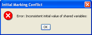
(a) Nonequal initial values error dialog. (b) Non-matching types error dialog.
</figure>
<xr id="fig:repjoin_join_errors" nolink />: Error dialogs related to the definition of Join nodes.


The Share All Similar Variables button joins all state variables in the children of the Join node with common names. The Join state variable will have the same common name. If you choose the names of submodels’ state variables appropriately with respect to the larger composed model, this feature proves very useful.

Delete Selected Variable(s) deletes the Join state variable selected in the left list. Delete All Shared Variables deletes all the Join state variables. The Sort additions to list checkbox controls how newly created state variables are added to the left list. If it is checked, the name of a new Join state variable will be added to the list in alphabetical order.


Replicate node

This node is a special case of the Join node. Its advantage over the Join node is that it leads to structural symmetries that can eventually result in less time- and space-consuming state-based numerical solution of the model. The extra restrictions that Replicate has relative to Join are as follows:

  • All children of a Replicate are of the same submodel type. Therefore, in the composed editor, a Replicate node is connected to only one child node, and the number of replications is specified in the Replicate node definition dialog.
  • Only state variables with the same name can be shared among replicas (copies) of a Replicate node. Therefore, to create a Replicate state variable, select only one state variable from the Replicate child; copies of that state variable will be shared among all replicas.

When you choose the Edit command from the context menu of a Replicate node, the Define Rep Node dialog, as shown in <xr id="fig:repjoin_rep_dialog" />, is shown. The label (name) of the Replicate node can be modified in the Rep Node Name edit box. The number of replicas can be set in the Number of Reps edit box. That number can be an integral constant or global variable that has been defined in the current composed model or in any of the constituent atomic or composed models. Two lists of state variables (called Unshared State Variables and Shared State Variables) and a number of buttons between them are used to move state variables from one list to the other.


<figure id="fig:repjoin_rep_dialog">

Repjoin rep dialog.png


<xr id="fig:repjoin_rep_dialog" nolink />: Replicate definition dialog.
</figure>


Each line in the latter (right) list shows the name of a state variable that has been shared among all replicas of the Replicate node. The rest of the state variables of the child submodel are shown in the left list. As mentioned before, each Replicate (or Join) node is itself a model. Notice that in the corresponding model of the Replicate node, for each name in the right list, there is only one copy of that state variable, and for each name in the left list, there are as many copies as have been specified in the Number of Reps edit box, i.e., one copy per child replica.

The buttons between the lists are self-descriptive. Share moves the selected state variable in the left list to the right list and Unshare does the reverse. Share All moves all state variables from the left list to the right list, and Unshare All does the reverse.


Graph

This section covers the overview of the Graph composition formalism supported in Möbius. It includes a brief description of the different parts of the Graph composed model editor and basic steps to build a composed model.

Overview

The Möbius tool also supports another composed model formalism called Graph composition[6] [7]. While the structure of a Replicate/Join composed model is an acyclic tree, the structure of a Graph composed model has no restrictions. Here, a Join node linking two models indicates an equivalence-sharing relationship between the two models, as in a Replicate/Join composed model. Much like Replicate/Join composition, lumping techniques based on computational group theory can be used to find all symmetries in the graph structure of the model automatically[6]. Exploiting these symmetries leads to efficiencies in the solution process. However, the graph theory used to detect these symmetries is currently not implemented in Möbius. Thus the Graph composition formalism, as it stands in Möbius, provides no advantage over the Replicate/Join composition formalism.

Graph composed model editor

<xr id="fig:repjoin_graph_faultyproc#1" /> shows the Graph composed model editor. As with other model editors, this editor can be opened either by creating a new model or by opening an existing one. To create a new Graph composed model, select Composed or any of its children in the project window and select the New command either by choosing it in the context menu or by clicking the leftmost icon in the toolbar (see <xr id="fig:project_main" />). To open an existing Graph model, select the Open command either by choosing it in the context menu or by clicking the corresponding icon. Because the Graph composed model editor is identical to the Replicate/Join composed model editor without a Replicate node, please refer to Section 5.1.2 for a discussion of this editor. As shown in <xr id="fig:repjoin_graph_faultyproc" />, any model expressed in the Graph composed model formalism can also be expressed in the Rep/Join formalism.

<figure id="fig:repjoin_graph_faultyproc">

<subfigure>Graph main editor.png</subfigure> <subfigure>Repjoin faultyproc.png</subfigure>
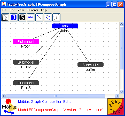
(a) Graph composed model editor. (b) The same model represented in the Rep/Join formalism.
</figure>
<xr id="fig:repjoin_graph_faultyproc" nolink />: A composed model represented in two different composition formalisms.


Action Synchronization

This section covers the overview of the Action Synchronization formalism supported in Möbius. It includes a brief description of the different parts of the Action Synchronization model editor and basic steps to build a composed model with this formalism.

Overview

The Möbius tool also supports the composed model formalism known as Action Synchronization. Much like the Replicate/Join composed model formalism, Action Synchronization takes the form of an acyclic tree, utilizing join nodes in a similar manner as Replicate/Join.

Action Synchronization is a composition formalism based on the notion of composing actions instead of places. If two actions are said to be shared between two models, then the new composed action’s enabling conditions are the union of the enabling conditions of the submodel actions, that is neither action can fire unless all are enabled. When the composed action fires, the result is then the union of results of the submodel actions.

Action Synchronization model editor

<xr id="fig:actionsync#1" /> shows the Action Synchronization composed model editor. The editor is accessed either by creating a new model, or opening an existing model, much as with the other composed editors.

<figure id="fig:actionsync">

<subfigure>Syncmaineditor.png</subfigure> <subfigure>Actionsyncjoin.png</subfigure>
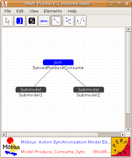
(a) Action Synchronization Model Editor. (b) Action Synchronization join node editor.
</figure>
<xr id="fig:actionsync" nolink />: Parts of the Action Synchronization Model Editor.


Due to the similarities of Action Synchronization to the Replicate/Join composed model editor, please refer to Section 5.1.2 for a discussion of most of the features of this editor. The primary difference comes when editing a join node itself.

Unlike the Replicate/Join composed model editor, Action Synchronization connects models by Joining on actions, not places. As such when the Join node editor (<xr id="fig:actionsync#2" />) is opened, instead of an option to “Create New Shared place”, we have “Create New Shared action”.

The shared action dialog, seen in <xr id="fig:actionsync_share" />, allows one to define synchronization amongst actions. Unlike sharing variables, shared actions need not have the same rate. The new shared action instead has the rate defined by the user in the “Rate” dialog. The actions to be shared in each of the submodels are then selected from the tabbed section of the dialog.


<figure id="fig:actionsync_share">

Definesharedaction.png


<xr id="fig:actionsync_share" nolink />: Shared action dialog.
</figure>


If the actions to be shared all have common names, the Share All Similar Action button can be used. If this is done the Join action will have the same common name. After sharing all similar actions, the shared actions must be edited with the Edit Selected action button to set the rate to an appropriate value.

Much as with the Replicate/Join editor, the button labeled Delete Selected Actions deletes the selected Join action from the list on the left, and Delete All Shared action deletes all of the Join actions.


Reward Formalisms

Reward formalisms define functions that measure information about the system being modeled. Currently, Möbius provides one reward formalism: performance variables.


Performance Variables

The Performance Variable Editor is shown in <xr id="fig:reward_main" />. It consists of a menu bar and a split pane. The left side of the split pane contains a tabbed panel with two tabs: Performance Variables and Model. The right side of the split pane contains the editable fields for the currently selected performance variable.


<figure id="fig:reward_main">

Reward main.png


<xr id="fig:reward_main" nolink />: Performance Variable Editor.
</figure>


The Performance Variables tab is the main display and is used to create new variables or select an existing variable so it can be edited, renamed, copied, or deleted.

The Model tab lists the top-level model on which this reward model is built. Often, the top-level model is a composed model, in which case the available submodels within the composed model are listed in the lower table. The top-level model is also referred to as child model of this reward model.

In addition to the menu options that are common to all Möbius editors (see Section 3.1), the following operations are available within the performance variable editor, via the main menu, buttons at the bottom of the left panel, or a right-click pop-up in the variable list:

  • Add Variable: Type the name of the new variable and click the Add Variable button (or hit the <Enter> key). The text in the new variable name text field disappears automatically when you type the new variable name.
  • Rename: Change the name of the selected variable.
  • Move Up: Move a variable up in the variable list. Allows for the grouping of related variables.
  • Move Down: Move a variable down in the variable list. Allows for the grouping of related variables.
  • Copy: Copy the selected variable to a new variable with a new name.
  • Delete: Delete the selected variable.

Variable definition

When a variable is selected in the variable list, the right side of the editor displays the variable definition panel. At the top of this panel is the name of the variable currently selected. Beneath the name is a tabbed pane used to define specifics of the variable. The tabbed pane contains five tabs: Submodels, Rate Rewards, Impulse Rewards, Time, and Simulation.

Submodels

The Submodels tab lists the names of all of the models in the child of the reward model. You must apply each reward variable to one or more of the available submodels. You can do so by selecting the model in the list. The <Ctrl> key can be used to select multiple individual items. The <Shift> key can be used to select a range of items.

When Möbius computes the reward function, it will do so on each instance of the selected models. For example, if there are N instances of the selected submodel in the top-level model, the reward function will be evaluated N times. For some types of reward functions, it is desirable to divide the reward function by the number of instances in the model (N in this example), so that the reward represents the average of the N instances.

With the current version of Möbius, you must use caution when defining rewards that depend on the state of multiple submodels. When multiple instances of the specified submodels are created by replication in the composed model, the results obtained are often nonintuitive. For example, consider a child model that is a composed model with 2 instances of submodel “A” and 3 instances of submodel “B”. If a reward is defined on state variables from both A and B, one might expect that the function would be evaluated five times (once on each A, and once on each B). However, that is not the case. Instead, the function will be evaluated a total of 6 times, once for each possible pair of an A with a B. (This behavior might change in future versions of Möbius.)

Selecting the submodel populates the Available State Variables panel in the Rate Rewards tab with the names of all state variables found in the selected submodel(s). Similarly, it also populates the Available Actions panel in the Impulse Rewards tab with all of the actions found in the selected submodel(s).

Rate rewards

The Rate Rewards tab is used to define rewards based on the time in each state. The top panel lists the Available State Variables, based on the submodels selected in the Submodels tab. The bottom panel contains the Reward Function. The reward function defines the measurement this rate reward should take. The reward function is written as a piece of C++ code, and should end with a return statement returning the value of the function.

As a shortcut for the user, double-clicking in the top panel inserts the state variable name at the location of the text cursor in the bottom panel. The value of the reward must be returned using the state variable value access function. This function is formalism-specific. For example, the value access function is Mark() for places in SANs and buckets in Buckets and Balls. Refer to the appropriate formalism documentation for details on access functions and other available functions that could be used to define rewards.

Impulse rewards

The Impulse Rewards tab defines reward functions that are evaluated when actions in the child model fire. The top panel contains a table showing the name of each action in the child model, and a column specifying whether or not an impulse function is defined for the action. To define an impulse function, click on the name of the function, and then write the C++ function for the impulse reward in the lower panel. The code should return the function result using the C++ return statement.


<figure id="fig:reward_impulse">

Reward impulse.png


<xr id="fig:reward_impulse" nolink />: Impulse reward definition.
</figure>


Impulse rewards can easily be used to count the number of times an action fires during an interval of time. To do so, set the impulse function to return 1, and set the type to Interval of Time with appropriate start and stop times (see next section).

Time

In order to solve for the reward measures via either simulation or numerical solution techniques, Möbius requires the specification of additional parameters for each reward variable. These parameters define the type of results to measure for the specific times of interest.

Reward variables can be defined as one of several different types. The type of the reward variable determines when, in system time, the reward function is evaluated. Evaluation times can be specified manually using a table, as shown in <xr id="fig:reward_time" />, or as an incremental range, as shown in <xr id="fig:reward_time_inc" />.


<figure id="fig:reward_time">

Reward time.png


<xr id="fig:reward_time" nolink />: Manual selection of time points for instant of time variable.
</figure>


<figure id="fig:reward_time_inc">

Reward time inc range.png


<xr id="fig:reward_time_inc" nolink />: Definition of time points using incremental range options.
</figure>


The possible reward variable types are:

  • Instant of Time: The reward function is evaluated at the specified point in time. The desired time is specified in the Start time field. Units of time are the same units used for the parameters for the action distributions in the atomic models.
  • Interval of Time: The variable returns the weighted sum of all of the values of the reward function, where each value is weighted by the amount of time the value is in existence, between the starting and ending times of the specified interval. The desired start and stop times for the interval are specified in the Start and Stop text fields.
  • Time Averaged Interval of Time: The variable returns the interval of time result, divided by the length of time for the interval. As with interval of time variables, the desired start and stop times for the interval are specified in the Start and Stop text fields.
  • Steady State: The reward function is evaluated after the system being modeled reaches steady state. The steady state simulation algorithm used is referred to in literature as batch means (see [8]). This approach assumes that there is an initial transient period that must pass before the system reaches its steady state behavior. Once the system is in steady state, the algorithm evaluates the reward function multiple times to gather the observations to compute the statistics. This technique is appropriate when enough time occurs between the samples to permit the assumption that the samples are independent of each other.
Simulation using batch means is typically more efficient than standard simulation approaches, since the possibly long initial transient period must be processed only once in batch means for all the observations, while traditional simulation would require processing of the initial transient period for each observation.

Simulation

The Simulation tab is used to define two aspects of reward variables that are unique to simulation. They are variable estimation and confidence interval definition.


<figure id="fig:reward_sim">

Reward sim.png


<xr id="fig:reward_sim" nolink />: Impulse reward definition.
</figure>


Estimation

When a model is being solved via simulation, the system is executed multiple times using different randomly generated event streams. Each execution generates a different trajectory through the possible event space of the system, due to the differences in the order and choice of events that occur. The reward variables are evaluated for each trajectory to create an observation. Statistical estimates of the reward variable value are then computed from the observations.

Multiple estimates can be computed for each variable. Möbius supports four basic estimations: mean, variance, the probability that the function is in an interval, and the probability distribution (and density) functions. To enable the computation of any of these types, click the appropriate check box. Additional parameters are required for intervals and distributions.

When Estimate Interval is selected, the four interface components beneath it are enabled. The Lower Bound and Upper Bound fields are used to specify the lower and upper bounds of the interval. The Include Upper (Lower) Bound checkboxes determine whether the upper (lower) bound itself is part of the interval.

When Estimate Distribution is selected, the four interface components beneath it are enabled. The Lower Bound and Upper Bound text fields specify the lower and upper limits of the distribution that will be measured. The Step Size determines the width of each bin in the discrete representation of the distribution. The number of samples in the distribution is computed by (Upper - Lower) / Step Size. Varying those three parameters makes it possible to focus distributions on specific areas of the reward function space, with varied resolutions. If Estimate out of range probabilities is selected, the probability that the reward function value will be lower than the lower bound of the distribution will be computed, as will the probability that the reward will be above the upper bound of the distribution.


Confidence

In order to get statistically significant estimations of the reward variables, it is necessary to generate many trajectories. In order to give an estimate of the accuracy of the calculated estimates, confidence intervals are computed as the observations are collected. When the simulation reaches the desired confidence level for every variable, the simulation will stop. (The simulator will also stop if it reaches a maximum observation limit without achieving the desired confidence level.)

Three parameters define the confidence interval. The Confidence Level text box specifies the desired probability that the exact value of the reward variable will be within the specified interval around the variable estimate. The Confidence Interval text box specifies the width of the acceptable interval around the variable estimate. The interval can either be Relative to the variable estimate, or be an Absolute number. For instance, a relative confidence interval of .1 and a confidence level of .95 for a mean variable will not be satisfied until the confidence interval is within 10% of the mean estimate 95% of the time.


Study Editors

Often a modeler wishes to investigate the behavior of systems for several different parameter values, perhaps corresponding to different system configurations. Möbius provides a convenient method to do so through the creation of studies. Recall from Sections 4 and 5 that global variables can be defined on atomic or composed models. A study allows one to examine the effect of varying parameters (global variables) on system performance. Within a study, one or more experiments may be defined based on the different values the parameters may take. More precisely, an experiment is one tuple of parameter values for which a model may be solved.

Möbius currently supports two types of studies: range studies and set studies. Keep in mind that even if no global variables have been defined in a model, a default study must still be created. A new study can be created by right-clicking on the Study node from the Möbius project tree view. The study editor selection dialog allows users to choose the appropriate types of study editor.


Range Study

A range study allows each global variable to be assigned either a fixed value or a range of values. In a range study, the experiments are created automatically by Möbius as the cross product of all possible values the global variables may take. For example, if there are two global variables, each of which is assigned a range of six values, the study will be composed of 36 experiments. The editor for a newly created range study is shown in <xr id="fig:studies_newrange" />. The name of each global variable defined in the child model is displayed in the table, along with its type and value (initially zero). You can reorder or resize the columns by clicking and dragging on the appropriate column header or border.


<figure id="fig:studies_newrange">

Studies newrange.png


<xr id="fig:studies_newrange" nolink />: New Range Study Editor.
</figure>


To enter a fixed value for a variable, simply click in the corresponding Variable Value text box and enter the value. To enter a range for a variable, click on the appropriate button at the bottom of the dialog (Incremental Range, Functional Range, Manual Range, or Random Range). An example of a completed range study can be found in <xr id="fig:studies_range" />. Note that if a variable is assigned a fixed value, that value is displayed in the table. Likewise, if a variable is assigned a range of values, the type of range is displayed.


<figure id="fig:studies_range">

Studies range.png


<xr id="fig:studies_range" nolink />: Completed range study example.
</figure>


Incremental range

An incremental range is specified with a starting value, an ending value, and an increment, which may be additive, multiplicative, or exponential. <xr id="fig:studies_incrange" /> shows the dialog. The first three elements of the dialog show the name of the study, the name of the variable being assigned, and the type of this variable.


<figure id="fig:studies_incrange">

Studies incrange.png


<xr id="fig:studies_incrange" nolink />: Incremental Range dialog.
</figure>


A variable defined with an incremental range will take on all values between Initial and Final at increments of Increment. That is, if a represents the initial value, b represents the final value, and i represents the increment, the variable will take on values for the different increment types according to <xr id="tab:studies_increments" />. Click on the View Values button to see a list of all the values the variable will take on in this range. The list may be exported to a text file.


<figtable id="tab:studies_increments">

<xr id="tab:studies_increments" nolink />: Three types of incremental ranges.
Increment Type Values
Additive a, a+i, a+2i, \dots, b
Multiplicative a, a*i, a*i^2, \dots, b
Exponential a, a^i, a^{i^2}, \dots, b
</figtable>


Functional range

A functional range is essentially a function of an incremental range. An incremental range is defined as in Section 7.1.1 to be the domain, and the functional range is obtained by applying a function to every element in the domain. Thus, the top half of the Functional Range dialog is identical to the Incremental Range dialog. The function may be a standard function, such as e^x or \sin x using the Range f(x) option, or a specialized function (e.g., quadratic, exponential, or linear) using the Range f(x,n) boxes.

For example, if the incremental range shown in <xr id="fig:studies_incrange" /> was used as the domain and f(x) = x^2 was used as the function, the result would be the dialog in <xr id="fig:studies_funcrange" /> and the values in <xr id="tab:studies_funcrange" />.


<figure id="fig:studies_funcrange">

Studies funcrange.png


<xr id="fig:studies_funcrange" nolink />: Functional Range dialog.
</figure>


<figtable id="tab:studies_funcrange">

<xr id="tab:studies_funcrange" nolink />: Functional range example.
Domain x Range f(x)
5.0 25.0
10.0 100.0
15.0 225.0
20.0 400.0
25.0 625.0
30.0 900.0
</figtable>


Manual range

Specify a manual range by entering each value in the range separately. To add a value to the range, enter the value in the New Value text box and click Enter. The values in the range are displayed in the Current Values box. The five buttons to the right of this box can be used to manipulate the values in the range as follows:

  • Up: Move a value up in the list
  • Down: Move a value down in the list
  • Delete: Delete the selected value from the list
  • Delete All: Delete all values in the list
  • Import: Import values from a text file

The incremental range in <xr id="fig:studies_incrange" /> could equivalently be represented by the manual range in <xr id="fig:studies_manrange" />. For this example, it would be more convenient to use an incremental range than to enter each value in the range manually. However, a manual range is necessary if you wish to specify range values that do not follow a regular pattern.


<figure id="fig:studies_manrange">

Studies manrange.png


<xr id="fig:studies_manrange" nolink />: Manual Range dialog.
</figure>


Random range

A random range allows you to assign random values to global variables. Enter into the Number of Samples text box the number of random values to generate within the range defined by Minimum Value and Maximum Value. <xr id="fig:studies_randrange" /> shows an example in which the variable arr_rate is assigned 6 random values between 5 and 30.


<figure id="fig:studies_randrange">

Studies randrange.png


<xr id="fig:studies_randrange" nolink />: Random Range dialog.
</figure>


Clicking the View Values button will display the pseuorandomly generated values, which may be exported to a text file. To create new values using a different seed, click the Regenerate button. The resulting values will be the actual values for the global variable used by the solver.


Set Study

A set study allows you to enter vectors of fixed values for each global variable. Thus, unlike a range study, in which experiments are created automatically, a set study has experiments that are defined explicitly by the user. Set studies are useful when the global variables do not change in a regular pattern with respect to each other. The editor for a newly created set study appears in <xr id="fig:studies_newset" />. All the global variables from the child model and their types are displayed in the table on the left. The Experiments table on the right shows the names of all the experiments that have been created as well as the values for the global variables in each experiment. Möbius requires that experiment names be distinct.


<figure id="fig:studies_newset">

Studies newset.png


<xr id="fig:studies_newset" nolink />: New Set Study Editor.
</figure>


When you create a new set study, one experiment is initially defined in which all global variables default to zero, as shown in <xr id="fig:studies_newset" />. To change the values of the global variables in an experiment, click inside the appropriate box in the column corresponding to the experiment and type the value. The buttons at the bottom of the dialog give you the ability to manage experiments, and are described in the following paragraphs.


Add     Click the Add button to add an experiment. Type the name of the new experiment at the prompt. Although the default name for the first experiment is “Experiment 1,” it can be renamed as explained below. In general, it may be helpful to give experiments more descriptive names.


Delete     To delete an experiment, click anywhere in the corresponding column of the Experiments table, and then click the Delete button. A prompt will ask you to confirm the deletion. Note that an experiment can be deleted only if multiple experiments exist in the study. If an experiment is the only one in the study, it cannot be deleted, since every study must contain at least one experiment.


Copy     To create a new experiment that has the same values for the global variables as an existing experiment, click anywhere inside the column for the original experiment and then click the Copy button. You will then be prompted for the name of the new (duplicated) experiment. While there would be no reason to have two identical experiments, using the Copy button is convenient when creating an experiment that is identical to another except for a few values, especially when the number of global variables is large.


Rename     Click the Rename button to rename an existing experiment. Type the new name of the experiment at the prompt and hit OK.


Import/Export     The Import and Export buttons are used, respectively, to import an experiment from a text file and export an experiment to a text file. The latter option requires that you select an experiment for export. The “import” function reads in files in the same format into which “export” writes them. Thus experiments may be exported for later import into a (possibly different) study in either Möbius or UltraSAN.


Experiment Activator

As mentioned previously, a study consists of one or more experiments. Both study editors include the ability to activate or deactivate experiments via the Experiment Activator button (see <xr id="fig:studies_set" />). To the left of this button in the dialog, the number of active experiments is displayed. An active experiment is one set of parameters for which the model will be solved when solution is performed (see Solving Models). In contrast, an inactive experiment will be skipped during solution. Use this function when only a subset of the experiments are to be carried out.


<figure id="fig:studies_set">

Studies set.png


<xr id="fig:studies_set" nolink />: Completed set study example.
</figure>


<xr id="fig:studies_expact" /> shows the dialog that will appear if you click the Experiment Activator button. At the top can be found the name of the study, the total number of experiments, and the number of them that are active. The table below lists the global variables and their values in each of the experiments. The check boxes underneath the experiment names indicate whether the experiment is active or inactive. All experiments are initially marked as active. To deactivate an individual experiment, click in the check box underneath its name. Click the Activate All or Deactivate All button to activate or deactivate all experiments at once. Then hit OK to commit or Cancel to discard changes.


<figure id="fig:studies_expact">

Studies expact.png


<xr id="fig:studies_expact" nolink />: Experiment Activator dialog.
</figure>


DOE Study Editor Interface

User Interface Flow

Section 1 presented the modeling flow in Möbius. The first steps in the modeling process are the definitions of the atomic, composed, and reward models. It is at these three modeling levels that all global variables are defined, but not assigned values. The study level is where global variables are assigned values. <xr id="fig:doe_flow_of_model_s" /> shows the modeling flow from the study level onward for a DOE study. During the study definition, all global variables are assigned values for each experiment. After a study is defined, it is saved and compiled into object code, which is later linked in by the solver during the model solution step. After all experiments are complete, the DOE study is reopened, and the results from the experiments are analyzed. If necessary, the study can be modified, and new experiments can be performed. This iterative process continues until the desired results are achieved. The remainder of this chapter will present the details of the graphical user interface of the DOE study editor.


<figure id="fig:doe_flow_of_model_s">

Doe flow of model s.png


<xr id="fig:doe_flow_of_model_s" nolink />: Flow of model solution with the DOE study editor.
</figure>


Defining a DOE Study

<xr id="fig:doe_flow_of_model_s" /> shows that the first step of the DOE experimentation process is to define a DOE study. There are several steps in the study definition process. <xr id="fig:doe_the_flow_of_eve" /> presents the flow of events involved in defining a DOE study. The remainder of this section will present the details of each step of the DOE study definition.


<figure id="fig:doe_the_flow_of_eve">

Doe the flow of eve.png


<xr id="fig:doe_the_flow_of_eve" nolink />: The flow of events in the DOE study definition process.
</figure>


The creation of a new DOE study is similar to the creation of any new model in Möbius. First, from the Möbius project window, select the type of module. Select the study node by clicking on the tree node named “Study” and then press the New button. A dialog asking for the study name and type is presented. <xr id="fig:doe_study_creat" /> shows a dialog from the creation of a study named “Workstation” of type “Design of Experiments Study.” After pushing the OK button, select the reward model upon which the study will be based. After selecting the appropriate reward model and pushing OK, you will be presented with the Constant Global Variable Selection dialog.


<figure id="fig:doe_study_creat">

Doe doe study creat.png


<xr id="fig:doe_study_creat" nolink />: DOE study creation dialog.
</figure>


The purpose of the Constant Global Variable Selection dialog is to help users select which global variables are to be held at constant values throughout the study. There are several reasons why some global variables would remain fixed to specific values during a study. One reason is that the variation of some model parameters may be relevant to another study, but not to the current one. Another reason to fix global variables to constant values is that a previous DOE study may have revealed that the variables do not significantly affect the reward model under study, so can be fixed to convenient values. Alternatively, the optimal values of some global variables may already have been determined from earlier studies. In that case, the global variables can be fixed to their optimal values. Any global variables that are held constant will not be included in the empirical model of the response created by the DOE analysis.

<xr id="fig:doe_constant_global" /> shows a Constant Global Variable Selection dialog with a list of all global variable names and types defined in the underlying model. To designate a global variable as constant, its checkbox in the Constant column must be selected by a single mouse click. Once that box has been selected, the value can be entered into the corresponding row under the Constant Value column. There are two ways to enter values into a table in the DOE study editor. One is to single-click the table cell and simply start typing the value. The other is to double-click the table cell. A blinking caret will appear, and all text will be left-justified while you are typing. Regardless of which method is used, pushing the <Enter> key will commit the new values to the table. After being entered, all numbers will be right-justified in their table cells. When all of the constant global variables have been selected, push the OK button to proceed to the next step. At any point during the study definition process, you may push the Cancel button in order to cancel the study definition process. After pushing the Cancel button, you will be asked whether the study is to be saved. If it is, it can be reopened later, and the definition process can resume. If you choose not to save the study, then it will be permanently discarded.


<figure id="fig:doe_constant_global">

Doe constant global.png


<xr id="fig:doe_constant_global" nolink />: Constant Global Variable Selection Dialog.
</figure>


The next step in the DOE study definition is the selection of the design type. <xr id="fig:doe_design_type_sel" /> shows the Design Type Selection dialog. The two categories of designs, factorial and response surface, are presented in separate tab panels. Selecting the Factorial tab shows a list from which either a Plackett-Burman or a two-level factorial design may be selected. Selecting the Response Surface tab displays a list with a choice of either a Central Composite or a Box-Behnken design. After selecting the desired design type from the appropriate list, you may either proceed to the next step by pushing the OK button, or return to the previous dialog by pushing the Back button. At any point in the study definition process, you may move forward or backward to any step and make changes to the study.


<figure id="fig:doe_design_type_sel">

Doe design type sel.png


<xr id="fig:doe_design_type_sel" nolink />: Design Type Selection dialog.
</figure>


After you have selected the design type, a dialog will prompt you to enter parameters for the chosen design. All design types require that both lower and upper bounds be specified for each nonconstant global variable. In factorial designs, global variables are varied over exactly two values. The values are equal to the low and high values entered in the design parameters dialog. <xr id="fig:doe_design_paramete" /> shows an example 2-Level Factorial Design Parameters dialog. The top table lists each nonconstant global variable name and type. A low and high bound must be entered for each variable. In two-level factorial and central composite designs, a second table displays a list of the different designs that are available. You should select the design that best suits the available computing resources. A single mouse click will highlight the row of the selected design. In <xr id="fig:doe_design_paramete" />, the full resolution design is selected. After all global variable bounds have been entered and the design fraction is selected, the study definition may proceed to the response selection step.


<figure id="fig:doe_design_paramete">

Doe design paramete.png


<xr id="fig:doe_design_paramete" nolink />: Design parameters dialog.
</figure>


A reward model may consist of several reward variables. Each of the reward variables can be solved using a variety of solution methods available in Möbius. For example, the mean and variance of a reward variable measuring workstation performance may be calculated by a simulation or via several numerical solution methods. The solution from each solver can be represented by a unique response. Each response can be analyzed separately, allowing for the comparison of different solution methods on the same reward variable.

<xr id="fig:doe_response_select" /> shows a Response Selection dialog. A checkbox near the top, labeled Edit responses separately for each reward variable, allows a different set of solution methods to be used for each reward variable. Usually, this checkbox is not selected, and all reward variables are solved using the same solution methods. A scrolling panel in the middle of the dialog lists all of the solver types available in Möbius. The user selects the desired solution methods by clicking the checkbox to the left of each solver name. At the bottom of the dialog window is a checkbox for selecting as a response the number of states in the state space. The purpose of the Response Selection dialog is to allow quick selection of a potentially large number of responses during an initial study definition. If desired, new responses can be added and existing responses deleted after the study definition process is complete.


<figure id="fig:doe_response_select">

Doe response select.png


<xr id="fig:doe_response_select" nolink />: Response selection dialog.
</figure>


DOE Study Editor Window

After a study is defined, the DOE Study Editor window appears. It is the main window and is always present, except during the study definition process. <xr id="fig:doe_study_edito" /> shows an example DOE Study Editor window. The data is from the fictitious workstation model from Sections 1 and 2. The window has four areas. The first is the menu bar at the top. The menu functionality will be discussed later in the chapter. At the bottom is the logo panel, which is similar to the logo panel found in other Möbius modules. The lower central portion of the logo panel contains a status area that occasionally displays messages in red text about the status of an activity.


<figure id="fig:doe_study_edito">

Doe doe study edito.png


<xr id="fig:doe_study_edito" nolink />: Response selection dialog.
</figure>


On the left side of the window is the design tree panel. The selected node of the design tree determines what is displayed in the main panel, which is the area directly to the right of the design tree. The design tree panel and main panel are separated by a movable divider. The mouse can be used to drag the divider left and right in order to give more screen area to a particular panel. At the top of the divider, as shown in <xr id="fig:doe_study_edito" />, there are two small triangles. Clicking one of the triangles moves the divider all the way to the edge of the window, causing either the design tree panel or the main panel to be hidden, depending on which triangle was clicked. If a panel is hidden, it can be revealed by a single click anywhere on the divider.

The graphical user interface for the DOE study editor was written using Java Swing classes. The appearance of the GUI varies depending on the operating system being used. The screen shots in this chapter were taken on the Microsoft Windows operating system. The DOE study editor will appear slightly different on other operating systems, such as UNIX or Linux. However, the functionality described in this manual will be consistent across operating systems.


Design Tree

Most of the time spent using the DOE study editor involves analyzing the contents of the main panel. There are five different views available for display in the main panel. Each of the five views corresponds to one of the five different types of nodes in the design tree. Clicking on an unselected design tree node will change the contents of the main panel. This section gives a brief description of each design tree node.

At the top of the design tree is the Notes node. Selecting the Notes node displays an editable text area in the main panel. Any comments entered in the text area will be saved when the study is saved. The text area supports cut, copy, paste, undo, and redo functionality, either from the Edit menu or by keyboard shortcuts. Cut, copy, paste, undo, and redo are performed by hitting <Ctrl>-<x>, <Ctrl>-<c>, <Ctrl>-<v>, <Ctrl>-<z>, and <Ctrl>-<Shift>-<z>, respectively.

Below the Notes node is the Design node, which, when selected, displays the design panel in the main panel. The design panel presents all input data for the study, including all global variable and response values for each experiment. The design panel will be discussed in Section 9.6.

Selecting the Summary node displays a design summary, an example of which is shown in <xr id="fig:doe_summary_panel" />. Response and global variable data are summarized in HTML-formatted tables. If the design is a two-level factorial type with less than full resolution, the alias structure is presented at the bottom of the summary panel. The text from the summary panel can be exported to a file using the Design menu’s Export Text menu item. Further details of all menu items will be offered in the next section.


<figure id="fig:doe_summary_panel">

Doe summary panel.png


<xr id="fig:doe_summary_panel" nolink />: Summary panel.
</figure>


The Analysis node contains a brief summary of the analysis procedure. Each response in the design panel has a corresponding tree node under the Analysis node. Response analysis requires several steps. Most of the functionality of the DOE study editor is used during response analysis. Before any analysis can be performed on a particular response, the user must enter response values for all experiments into the design panel. Details on how to do so will be presented in Section 9.6.


Menus

There are four menus in the DOE study editor. The first is the File menu, which performs the same functions as the File menus in other Möbius editors. The Save item saves any changes to the study to disk and compiles the global variable values for each experiment into object code. A dialog appears that shows the progress of the compilation and linking process. The object code will be linked in by the solver during model solution. The Document menu item saves an HTML description of the study in the study directory. The Close menu item closes the DOE study. If any changes were made, you will be prompted to decide whether the changes should be saved.

The Edit menu provides basic cut, copy, and paste functionality in any editable text area or text field. Undo and redo functionality are also available, but only in the notes panel, as discussed earlier. Keyboard shortcuts are available for all menu items.

The Design menu contains items specific to the DOE study editor. The Export Regression Model menu item is only enabled when an appropriate analysis panel is displayed. The uses of exporting the regression model will be discussed in Section 8.8.2.

The Export Text menu item is used to save any displayed panel to a text or HTML-formatted file. If the notes or design panel are displayed, the contents of the panel will be saved to a text file. If the summary panel is displayed, the contents of the panel will be saved to an HTML file. Other uses of the Export Text menu item will be presented later.

The Redefine Design menu item is used to initiate the study definition process explained in Section 8.2. A user might wish to redefine a study to correct a mistake made during the initial study definition. He or she could also use redefinition to augment the design. Design augmentation involves adding more experiments to a study so that more information can be gained about the responses under study. For example, a half-fraction two-level factorial design may not present enough information for the user to build an accurate empirical model of the response. The design can be augmented with the other half-fraction in order to create the full-resolution design, doubling the number of experiments in the study. However, half of the experiments will already have been completed. After the remaining half are run, an analysis of the full resolution 2k design can be performed. One caveat of design redefinition is that all data in the response columns in the design panel are erased when a study is redefined. In order to restore the data, the user must re-query the results database to fill in the response columns. Instructions for gathering response data from the results database will be presented in the next section.

The Hide/Show Logo Panel menu item is useful for gaining valuable screen area. On small screens, it may be difficult to view some of the graphs in the analysis panels. Hiding the logo panel can increase the area available for viewing such graphs. That can reduce the amount of scrolling necessary in viewing the data. One disadvantage of hiding the logo panel is that the status bar will not be visible; furthermore, any important messages displayed there would also not be visible.

The last item in the Design menu displays a list of preferences for the current study. <xr id="fig:doe_preferences_dia" /> shows an example Preferences dialog. The first two items allow the user to specify the preferred window dimensions. Once the preferred height and width have been entered and the study has been saved, the DOE Study Editor window will reopen with the specified window dimensions. This feature allows users to customize the window size to suit a particular large or small screen. The remaining preference items are specific to the analysis procedure and will be discussed later. It is important to note that saved preferences are relevant only to a specific study, not to all DOE studies.


<figure id="fig:doe_preferences_dia">

Doe preferences dia.png


<xr id="fig:doe_preferences_dia" nolink />: Preferences dialog.
</figure>


The last menu is the Help menu on the right side of the menu bar. The About item displays information about copyrights and contact information for the PERFORM research group. The Reward Info item displays the name of the reward model on which the study is based.


Design Panel

Whenever a DOE study is opened, the first view displayed in the main panel is the design panel. The design panel displays the entire experimental design in the design table. <xr id="fig:doe_design_table" /> shows an example design table. Each row represents an experiment. The global variable columns represent the factor values. The reward variable columns represent the responses. The Active column displays the experiments that will be performed by the solver, and replaces the Experiment Activator found in the Set and Range study editors. If a checkbox is selected, then the experiment for the corresponding row is active.


<figure id="fig:doe_design_table">

Doe design table.png


<xr id="fig:doe_design_table" nolink />: Design table.
</figure>


You can activate several pop-up menus by right-clicking on certain column headers of the design table. The Active column has a pop-up menu with four choices for experiment activation. All experiments can be either activated or deactivated with a single menu choice. Alternatively, experiments from only the selected rows can be activated or deactivated. Row selection is performed by left-clicking on a row with the mouse. The <Shift> and <Ctrl> keys can be used with the mouse click to select a sequence or noncontiguous block of rows, respectively.

For response surface designs, a pop-up menu is available on the Experiment column header. The user may add experiments to the bottom of the table. Any user-added experiments may be removed from the table via the Remove Selected item on the Experiment column’s pop-up menu. Only user-added experiments may be removed from the design table; the built-in design must remain intact. The ability to add experiments to factorial designs is not enabled. The factorial designs built into Möbius are orthogonal. Adding arbitrary experiments would destroy the orthogonality and distort the analysis. Response surface designs do not require orthogonality for analysis. You should avoid creating arbitrary experiments that are far from the design space of the original built-in design. Points far from the original design center can grossly distort the response surface, resulting in inaccurate prediction. For the same orthogonality reason, global variable values cannot be edited in the design table for factorial designs. They can, however, be edited in response surface designs. Again, you are cautioned against entering factor levels that produce design points far from the original design.

You can activate the response pop-up menu by right-clicking on any reward variable column header. The Insert Response item allows you to add a single response column to the table. The dialog in <xr id="fig:doe_response_insert" /> appears, prompting you to select the reward variable, the solver type, and the reward type. Pushing the OK button in the example shown in <xr id="fig:doe_response_insert" /> would add a new response measuring the mean performance using the adaptive transient solver. The Delete Response item removes a response column from the table. There must be at least one response, so the last response cannot be deleted.


<figure id="fig:doe_response_insert">

Doe response insert.png


<xr id="fig:doe_response_insert" nolink />: Response insertion dialog for design table.
</figure>


There are three menu items in the response pop-up menu associated with filling the column with data. One item, which is very useful for experimenting with the DOE study interface, is the Fill With Random item. Selecting that menu item will fill the response column with uniformly distributed integers between 90 and 110. No analysis of a response can take place until the entire response column is filled with data. Therefore, the Fill With Random feature is a quick way to start playing with the analysis tools, which will be described later. To analyze real data, you must fill the response columns with solver data by querying the results database for the model solutions.

There are two pop-up menu items for filling a response column with data from the results database. The Fill Selected item fills in data only for the selected rows in the design table. The Fill Column item fills the entire column with the solved reward variable results. Selecting either of the two choices causes a dialog similar to the one in <xr id="fig:doe_solver_selectio" /> to appear. Because the column associated with the pop-up menu represents data from a simulator, the dialog in <xr id="fig:doe_solver_selectio" /> will prompt you to select from a list of simulators defined in the project. Once the solver has been selected, the results database will be queried, and the response values will be retrieved and placed into the response column.


<figure id="fig:doe_solver_selectio">

Doe solver selectio.png


<xr id="fig:doe_solver_selectio" nolink />: Solver selection dialog for results database query.
</figure>


To erase values from a response column, the Clear Selected or Clear Column pop-up menu items can be selected. The Clear Selected item clears the response values only for the selected rows in the table. The Clear Column item erases the entire column. The user may also edit the response values by typing the values directly into the table cells. Only after every response value in a column has been entered may analysis of the response be performed.


Analysis Procedure

For every response column in the design table, there is a corresponding node under the Analysis node in the design tree. After all response values have been filled in for a particular response column, the corresponding tree node can be activated. Clicking on the response node reveals the analysis tabs in the main panel. There is a sequence of six tabs that, when clicked, reveal a panel for performing one step in the analysis procedure. The user interface for the tab panels will be presented in the remainder of the chapter. <xr id="fig:doe_analysis_flow_i" /> shows the analysis flow corresponding to the six tab panels. In summary, the goal is to build and evaluate a regression model of the response and to use the regression model to predict response values at points in the design space other than the experimental points. Steps 1 and 2 transform the observed response values (if necessary) and build a regression model from the significant effects. Steps 3 and 4 analyze the model for significance and test the assumptions made on the data. If the model is good, then it can be used to produce graphs of the response and predict new values in the design space, as indicated in steps 5 and 6 of <xr id="fig:doe_analysis_flow_i" />. The six tabs are shown along the top of <xr id="fig:doe_six_tab_panels_" />. They progress from left to right as the analysis progresses.


<figure id="fig:doe_analysis_flow_i">

Doe analysis flow i.png


<xr id="fig:doe_analysis_flow_i" nolink />: Analysis flow in the DOE study editor.
</figure>


<figure id="fig:doe_six_tab_panels_">

Doe six tab panels .png


<xr id="fig:doe_six_tab_panels_" nolink />: Six tab panels in analysis procedure with Transformation tab selected.
</figure>


The first step in the analysis procedure allows the user to transform the observed response values. After a transformation is applied, all analysis is done on data that are some function of the original solver values. There are three situations in which a transformation may be required. The first occurs when the maximum-to-minimum ratio of the response values is large. The second occurs when a priori knowledge of the system results in the belief that a particular function of the response, rather than the response itself, is better suited to a regression model. Both of those situations require that the transformations take place before any analysis is performed. It is for that reason that the Transformation tab is placed first in the analysis flow.

The third situation in which a transformation is required occurs after an initial analysis has revealed that the assumptions on the response data have been violated. For example, a nonconstant variance might not be discovered until the Diagnostic Plots phase of the analysis. The user must then backtrack to the Transformation tab, build a new regression model, and re-analyze the data. It is very common to move backward and forward while experimenting with different model parameters. The interface allows the user to click on a previous tab at any time to try out new settings. Regression model analysis is often trial-and-error because the underlying model of the response behavior is unknown. The whole point of experimental design is to allow better understanding of the structure of the response.

<xr id="fig:doe_six_tab_panels_" /> shows the list of available transformations on the left side of the transformation panel. Selecting any transformation changes the graphic to the right of the transformation list. The first seven transformations belong to the power family. The graphic for each power transformation contains a sample of what the Residuals vs. Predicted Response plot should look like if the selected power transformation is applicable. All graphics contain information about when the selected transformation is most useful. Most transformations have restrictions on the input data, which are illustrated in each transformation’s graphic. Many transformations have optional parameters that can be entered in the text fields that appear below the transformation list when appropriate. The most common parameter is the translation constant c. Adding the appropriate constant to each reward variable will translate the values to a range for which the selected transformation is valid. If the selected transformation is invalid for any response values, a dialog will warn about the offending values when the user tries to progress to the next analysis step. The ratio of maximum-to-minimum response values is presented below each graphic to aid in the decision on whether a transformation is necessary.

Most commonly, no transformation is applied to the response. The remaining analysis steps are identical regardless of whether the response has been transformed. If you do use a transformation, it is important for you to remember that regression model plots and prediction are presented in the transformed domain. Whenever possible, the response is labeled wrapped in the corresponding transformation function. For example, if the natural logarithm transformation is used, the response will be labeled “Ln[response_name].”


Model Selection

After the appropriate transformation has been selected, the next step is to click on the Model tab and choose the effects to include in the regression model. The method for choosing effects varies depending on whether a factorial or a response surface design is being analyzed. Each case will be presented separately.

Factorial model selection

For factorial designs, one may select effects either graphically or from a table. Each selection interface has a separate tab panel within the model panel. The Normal Plots tab shows the normal quantile plot of effects. <xr id="fig:doe_normal_plot_of_" /> shows an example normal plot of effects. If the effects follow a normal distribution, then the normal quantile plot of ordered effects will follow a straight line. The outliers are the significant effects. On the normal plot of effects, outliers appear at the top and bottom of the plot. <xr id="fig:doe_normal_plot_of_" /> shows three outliers: two at the top and one at the bottom. To select an effect for inclusion in the regression model, the user simply clicks the point corresponding to the effect. The selected points will turn from blue to red, and the label of the chosen effect will be placed near the selected point. An ordinary least squares straight line will be drawn through all unselected blue points.


<figure id="fig:doe_normal_plot_of_">

Doe normal plot of .png


<xr id="fig:doe_normal_plot_of_" nolink />: Normal plot of effects for factorial design.
</figure>


The most common graphical method for selecting effects is the half-normal plot. The half-normal plot is identical to the normal plot, but the absolute values of the effects are plotted. All outliers appear in the top right section of the plot. <xr id="fig:doe_half_normal_eff" /> shows the same data as <xr id="fig:doe_normal_plot_of_" />, but plotted on a half-normal quantile plot. All three outliers (largest effects) are selected at the top right of the plot. In this example, main effects B, E, and G are included in the regression model.


<figure id="fig:doe_half_normal_eff">

Doe half normal eff.png


<xr id="fig:doe_half_normal_eff" nolink />: Half normal effects plot.
</figure>


You may switch back and forth from normal to half-normal views of the effects plots by selecting the appropriate button under the factor list at the left side of the normal plots panel. You can unselect all selected points by pressing the Clear Selection button. The Fill Points checkbox controls whether the plotted points are filled-in colored disks, or simply hollow circles. Deselecting the checkbox can make point labels easier to read on a very crowded plot.

The user can also select effects via the table in the Effects tab panel. <xr id="fig:doe_factorial_effec" /> shows the effects table corresponding to the data in the normal plots in <xr id="fig:doe_normal_plot_of_" /> and <xr id="fig:doe_half_normal_eff" />. Only the portion of the table listing the nonaliased effects is shown, in order to conserve space. The first column lists all effects up to five factor interactions. You can include in the regression model any effect that is not aliased by clicking on the corresponding checkbox in the In Model column. The next two columns list the effect estimate and sum of squares value for each effect. If an effect is aliased, the word “aliased” appears instead of a sum of squares value. The % Contribution column lists the percentage that the corresponding effect’s sum of squares contributes to the total sum of squares. The elements of the % Contribution column will always add to 100%, except in Plackett-Burman designs in which interactions contribute a nonzero sum of squares. Only main effects are listed for Plackett-Burman designs. The last column lists the aliases of the effects in the first column. Only aliases for up to five factor interactions are listed. A complete list of the alias structure can be found in the Summary tree node.


<figure id="fig:doe_factorial_effec">

Doe factorial effec.png


<xr id="fig:doe_factorial_effec" nolink />: Factorial effects table.
</figure>


Each column in the effects table is sortable. Clicking on any column header will sort the list in descending order. Clicking again will sort in ascending order. The standard procedure is to click on the % Contribution column header to bring the effects that explain the most observed variability of the response to the top of the column. Effects with larger percent contributions are more likely to be significant regression model terms. <xr id="fig:doe_factorial_effec" /> shows that the top three effects, E, G, and B, are selected for inclusion in the regression model. Those effects were also selected in the normal plots in <xr id="fig:doe_normal_plot_of_" /> and <xr id="fig:doe_half_normal_eff" />. Selecting an effect from the effects table is equivalent to selecting the same effect from the normal plot.

The effects table in <xr id="fig:doe_factorial_effec" /> shows that effects E and G explain 52.7% and 33.3% of the observed variability of the response. Suppose that experience with the system being modeled indicates that the interaction EG should exert a strong effect on the response. Suppose also that factor B is not expected to be influential on the response. However, according to the effects table, B explains 13.9% of the observed variability. Careful inspection of the aliases for effect B reveals that B is aliased to EG (and several other interactions). This observation would lead the experimenter to conclude that the 13.9% variability is due to interaction EG, not factor B. Inclusion of factor B in the regression model would lead to invalid conclusions. Fortunately, there is a way to alter the alias arrangement in the effects table so that the correct effect can be added to the regression model.

Right-clicking on any row of the Effect or Aliases column activates a pop-up menu allowing the aliases for the row’s effect to be edited. <xr id="fig:doe_edit_aliases_di" /> shows the dialog that appears after a user has selected the pop-up menu item to edit the aliases for effect B. The pop-up shows a pull-down menu listing the aliases of B. After term EG has been selected, the effects table is updated as shown in <xr id="fig:doe_updated_effects" />. Factors E, G, and their interaction EG will then be used to build the regression model.


<figure id="fig:doe_edit_aliases_di">

Doe edit aliases di.png


<xr id="fig:doe_edit_aliases_di" nolink />: Edit aliases dialog.
</figure>


<figure id="fig:doe_updated_effects">

Doe updated effects.png


<xr id="fig:doe_updated_effects" nolink />: Updated effects table after aliases have been edited.
</figure>


Regression models in the DOE study editor are required to be hierarchical. In a hierarchical model, all parent effects for all interactions in the model must also be included in the model. For example, if interaction ABC is included in a regression model, the parent effects A, B, C, AB, AC, and BC must also be included. Möbius automatically includes the terms necessary to make the selected model hierarchical. This automatic update is performed whenever the user switches to a different view in the main panel. Clicking from the Effects tab to the Normal Plots tab will automatically cause all parent effects to be added to the selected regression model.

Response surface model selection

The method of effect selection for response surface designs differs from the factorial method. There is no graphical procedure for selecting effects for response surface designs. Under the Model tab in response surface designs, there are two tabs to choose from: the Fit Summary and Model Selection tabs.

The fit summary panel summarizes the fit of several regression models to the observed response values. An ANOVA table is used to calculate the significance of each model. <xr id="fig:doe_anova_table_in_" /> presents an example ANOVA table for five models. The mean regression model contains only the average response value. If \beta_0 is the average, then the model is simply y=\beta_0. The linear model contains the mean and all main effects. The two-variable interaction model contains all effects from the mean and linear models, plus all two-factor interactions. Each successive model adds more terms to the model. The quadratic model adds pure second-degree effects (A2, B2, C2\ldots). The cubic model adds all pure cubics (A3, B3, C3\ldots), all mixed terms (A2B, A2C, AB2\ldots), and all three-factor interactions (ABC). The ANOVA is calculated using the sequential sum of squares method explained in Section 3.5. The Significant column in the ANOVA table tells whether the corresponding model’s additional terms added to the sequential model contribute significantly to the observed variability in the response. From <xr id="fig:doe_anova_table_in_" />, it is clear that the pure quadratic terms contribute significantly to the regression model. The linear and two-variable interaction models are not significant. The response surface must exhibit second-order characteristics, which are best modeled with quadratic regression polynomial terms.


<figure id="fig:doe_anova_table_in_">

Doe anova table in .png


<xr id="fig:doe_anova_table_in_" nolink />: ANOVA table in fit summary panel.
</figure>


A second table of model statistics presents further information to help users choose appropriate regression models. <xr id="fig:doe_fit_summary_mod" /> lists useful statistics for each of the models presented in the ANOVA table in <xr id="fig:doe_anova_table_in_" />. The Adjusted R^2 column is the most important. The table exhibits the fact that the R^2 value always increases as terms are added to the regression model, but the adjusted R^2 can actually decrease. A negative adjusted R^2 for the linear and two-variable interaction models indicates that they are not adequate models of the response. The quadratic model explains 74.59% of the response’s observed variability, according to the adjusted R^2 value.


<figure id="fig:doe_fit_summary_mod">

Doe fit summary mod.png


<xr id="fig:doe_fit_summary_mod" nolink />: Fit summary model statistics table.
</figure>


In both example fit summary tables, the cubic model is aliased. The concept of an aliased model in response surface methodology is similar to that in factorial designs. An aliased model is one in which there have not been enough experiments performed to estimate all of the effects in the model. In order to de-alias a response surface model, it is necessary to add more experiments in the design panel, as explained in Section 8.6.

The last piece of information presented in the fit summary panel is the sum of squares details for the ANOVA table. Each effect added to the sequential model has a corresponding sum of squares term. There are two separate sum of squares lists. The first is sorted by effect name; the second is sorted in descending order by sum of squares magnitude. The most influential effects will be placed at the top of the second list. It is important to remember that for a sequential sum of squares, the order in which effects are added to the model may affect the magnitude of the sum of squares. The sorted sum of squares list is useful for selecting potentially highly significant effects for inclusion in the regression model.

Effects are added to the regression model in the model selection panel. The table in <xr id="fig:doe_model_selection" /> lists each effect in the first column and a corresponding checkbox in the second column. A single mouse click on the checkbox toggles the effect’s inclusion in the model. When any row is selected, the user can activate a pop-up menu by right-clicking anywhere on the table. The pop-up menu, shown in <xr id="fig:doe_model_selection" />, contains items for removing all selected effects from or adding all selected effects to the regression model. An alternative to clicking directly on the table to select effects is to use the Model pull-down menu above the table. From the pull-down menu, the mean, linear, quadratic, cubic, or other model may be selected.


<figure id="fig:doe_model_selection">

Doe model selection.png


<xr id="fig:doe_model_selection" nolink />: Model selection effects table.
</figure>


By default, the highest-degree effect listed in the model selection panel is three. You can alter this maximum degree by selecting a different maximum degree from the preferences dialog. The choices for the maximum degree are two through six. Another way to add a specific higher-order effect to the table is to type the desired effect in the text field at the top of the Model selection panel and click the Add Effect button. For example, if effect A5B is desired, the user may type any of “A5B”, “a5b”, “A5B”, or “a5B” and push the Add Effect button to place A^5B in the table. All parent effects required to support hierarchy are automatically added to the table. Therefore, adding A5B will automatically add A^4, A^3B, A^5, and A^4B to the table if they are not already there. The maximum degree effect allowed is six. For example, AB^2C^3, ABCDEF, and A^6 are all sixth-degree effects. To remove any user-added effects, you can press the Remove Effect button; a dialog will prompt you to select from a list of added effects. The selected effect and all parent effects required for hierarchy are then removed from the table.

By default, no exponents of degree four or higher are displayed in superscript font. If the computer system running the Möbius interface has the superscript fonts installed, then you can activate their display by clicking the Use Exponent Font in Effects checkbox in the preferences dialog. Selecting this option also affects the display of exponents in the fit summary and ANOVA panels.

ANOVA

After the effects for the regression model have been selected, a statistical analysis can be performed to evaluate the quality of the model. Clicking on the ANOVA tab reveals a wide variety of statistical output about the regression model. <xr id="fig:doe_initial_data_in" /> shows the first four pieces of information from an example response surface design. The first two items summarize the response and transformation information. The next two items do not always appear. If effects had to be automatically added to the regression model in order to make it hierarchical, then a list of those effects will be presented below the transformation data, as presented in <xr id="fig:doe_initial_data_in" /> . The final piece of data applies only to response surface designs. It is possible in the model selection panel to select more effects than can be independently estimated given the available degrees of freedom. If this happens, some of the selected effects will be aliased to other effects in the model. As effects are sequentially added to the regression model from lower to higher order, any effect that is aliased to an effect already in the model is not actually added to the model. Instead, it is placed in the list of aliased terms presented in the ANOVA panel. The alias structure is dependent on which effects are already in the model. Therefore, the complete alias structure for the selected model is presented in the ANOVA panel after the entire model is selected.


<figure id="fig:doe_initial_data_in">

Doe initial data in.png


<xr id="fig:doe_initial_data_in" nolink />: Initial data in ANOVA panel.
</figure>


The next item in the ANOVA panel is the analysis of variance table. <xr id="fig:doe_anova_table_wit" /> shows a screen capture of the ANOVA table for a typical Möbius model. The significance of the model and each effect should be analyzed. If an effect is not significant and it is not required to support the model hierarchy, then it should be removed from the model. The significance and insignificance thresholds are defined in the preferences dialog. The default thresholds are 0.05 for significant and 0.1 for insignificant. Any effect with a P-Value less than the significance threshold is significant. Any effect with a P-Value greater than the insignificance threshold is not significant. The significance of an effect with a P-Value between the two thresholds is left to the experimenter to decide.


<figure id="fig:doe_anova_table_wit">

Doe anova table wit.png


<xr id="fig:doe_anova_table_wit" nolink />: ANOVA table with summary.
</figure>


A summary of the ANOVA results is presented after the ANOVA table. The summary in <xr id="fig:doe_anova_table_wit" /> gives an interpretation of the model P-Value. Multiplying the model P-Value by 100 gives the percent possibility that the given significance level could occur strictly by chance. A summary of which terms are significant and not significant is also given.

After the ANOVA summary, there are two tables of regression model statistics. The theory behind these statistics was presented in Section 3.6. <xr id="fig:doe_regression_mode" /> shows a sample with a summary of the data below the tables. The adjusted R2 should be as close to one as possible. The model should explain as much variability as possible without insignificant effects. The prediction capability of the regression model is best when the adjusted R2 and prediction R2 are as close to each other as possible. If the two are within 0.20 of one another, then the predictive quality is acceptable.


<figure id="fig:doe_regression_mode">

Doe regression mode.png


<xr id="fig:doe_regression_mode" nolink />: Regression model statistics table.
</figure>


A table of diagnostic statistics for each experiment is presented next. The data in each column are presented graphically in the Diagnostic Plots panel. The tabular presentation is an alternative to the scatter plots and is preferable for some users. For experiments with leverage values of one, the student’s residuals, Cook’s distance, and outlier t are undefined.

Below the diagnostic statistics table are two representations of the regression model polynomial. <xr id="fig:doe_regression_equa" /> shows both representations. Each polynomial is written with one term per line to facilitate formatting. For example, the first equation in <xr id="fig:doe_regression_equa" /> is


Performance.mean=5.25+1.5A+0.75B+0.5AB


The first equation is presented in coded global variable terms. The coded variables are the natural values scaled from –1 to +1. They are the values used for internal calculations. The equation in terms of natural global variable values is the one used to predict response values. The first item in the Design menu allows the natural form of the regression equation to be exported to a file. The file may be in either plain text or Mathematica notebook format.


<figure id="fig:doe_regression_equa">

Doe regression equa.png


<xr id="fig:doe_regression_equa" nolink />: Regression equations in coded and natural formats.
</figure>


The final piece of data presented in the ANOVA panel is a table of standard errors and confidence intervals for each regression model coefficient. <xr id="fig:doe_standard_errors" /> shows an example table. The standard error is the standard deviation of the coefficient estimate. The 95% confidence intervals represent the range in which the coefficients should lie 95% of the time. If the range contains zero, then the coefficient is not significant.


<figure id="fig:doe_standard_errors">

Doe standard errors.png


<xr id="fig:doe_standard_errors" nolink />: Standard errors and confidence intervals for regression coefficients.
</figure>


The area of the ANOVA panel containing the table of standard errors is an editable text area. Comments can be entered in the text area. The entire ANOVA panel can be exported to an HTML file using the Design menu’s Export Text item. A plain-text version of the ANOVA table can also be appended to the ANOVA panel output if the appropriate checkbox is selected in the preferences dialog. The plain-text version is useful for copying and pasting text into the notes panel or to another application.


Diagnostic Plots

If the regression model produced satisfactory results in the ANOVA panel, the analysis may proceed to the Diagnostic Plots panel. The diagnostic plots consist of six scatter plots of the data from the Diagnostic Statistics table in the ANOVA panel. Six buttons on the left side of the Diagnostic Plots panel control which of the six plots is displayed. <xr id="fig:doe_normal_plot_of_" /> shows the panel with an example normal plot of studentized residuals. Each point in the diagnostic plots can be selected with a single mouse click. An information panel above the buttons gives details about the selected point, such as the coordinates and the corresponding experiment number.

The normal plot of studentized residuals in <xr id="fig:doe_normal_plot_of_stud" /> shows that the response residuals generally follow a straight line throughout the central portion of the plot. Therefore, it can be assumed that the residuals are normally distributed. The outliers at the lower and upper extremes are not sufficient grounds for dismissal of the normality assumption. The outlier in the upper right portion of the plot is selected in red. The information panel reveals that the selected outlier corresponds to experiment 45.


<figure id="fig:doe_normal_plot_of_stud">

Doe normal plot of stud.png


<xr id="fig:doe_normal_plot_of_stud" nolink />: Normal plot of studentized residuals.
</figure>


Clicking on the Residuals vs. Predicted button reveals the plot in <xr id="fig:doe_student_residua" />. With the exception of the selected outlier, no visible trend is present. Therefore, the assumption of constant variance of residuals is valid. As in the previous plot, the outlier corresponds to experiment 45. A checkbox below the six plot selection buttons toggles the display of studentized residuals versus ordinary least squares residuals. The studentized form of residuals is preferred. However, in some cases, the studentized residuals are not defined. In those cases, the ordinary residuals must be used to validate the assumptions.


<figure id="fig:doe_student_residua">

Doe student residua.png


<xr id="fig:doe_student_residua" nolink />: Student residuals vs. predicted response diagnostic plot.
</figure>


The Predicted vs. Actual plot in <xr id="fig:doe_predicted_vs__a" /> shows that most points are gathered near the 45o line, implying a fairly good least squares fit. The point farthest from the line is selected in red and, again, corresponds to experiment 45. The data gathered from the first three plots indicate that experiment 45 may have a problem.


<figure id="fig:doe_predicted_vs__a">

Doe predicted vs a.png


<xr id="fig:doe_predicted_vs__a" nolink />: Predicted vs. actual diagnostic plot.
</figure>


The outlier t plot in <xr id="fig:doe_outlier_t_diagn" /> shows that experiment 45 is indeed an outlier. The information panel indicates in red type that the value of the outlier t for experiment 45 is barely larger than 3.5, making it an outlier. Further investigation by the experimenter would be required in order to either justify or discount the data from the outlying experiment.


<figure id="fig:doe_outlier_t_diagn">

Doe outlier t diagn.png


<xr id="fig:doe_outlier_t_diagn" nolink />: Outlier t diagnostic plot.
</figure>


The leverage plot in <xr id="fig:doe_leverage_diagno" /> shows a pair of points with leverage values greater than twice the average leverage value. The two points exert a disproportionately large influence on the model fit. The Cook’s distance plot in <xr id="fig:doe_cook___s_distan" /> does not reveal any evidence of disproportionately large influence among the experimental points. Any points that cross the threshold lines in the leverage or Cook’s distance plots should be investigated.


<figure id="fig:doe_leverage_diagno">

Doe leverage diagno.png


<xr id="fig:doe_leverage_diagno" nolink />: Leverage diagnostic plot.
</figure>


<figure id="fig:doe_cook___s_distan">

Doe cook s distan.png


<xr id="fig:doe_cook___s_distan" nolink />: Cook’s distance diagnostic plot.
</figure>


If all diagnostic plots look good, then the analysis may proceed to the inspection of the regression model graphs. If any of the diagnostic plots reveal a problem, then the analysis should not proceed to the next step. Instead, transformations, model reduction, or additional experiments should be considered. Conclusions from the Model Plots and Prediction phases of the analysis are valid only if all diagnostic tests show satisfactory results.

After verifying that the regression model is adequate for prediction, the user can use plots of the regression model to analyze response behavior. There are five different types of plots available in the model plots panel. The user selects the type of plot by clicking on the appropriate tab within the model plots panel. All of the plot panels have the same layout. <xr id="fig:doe_one_factor_mode" /> shows the layout of the one-factor plot panel. The plot occupies the right side of the panel. The left middle portion of the panel contains slider controls for each global variable in the regression model. A slider can be enabled or disabled. If a slider is disabled, it will appear dimmed. In <xr id="fig:doe_one_factor_mode" />, the slider for global variable A:Memory_RAM is disabled, but the other two sliders are enabled. A slider becomes disabled when its corresponding global variable is selected as an axis label. In <xr id="fig:doe_one_factor_mode" />, the horizontal, or x-axis, is labeled as A:Memory_RAM. Axes are selected from pull-down menus at the bottom left corner of the main panel. An information panel above the sliders displays the axes labels and the current values of all factors corresponding to all enabled sliders. In <xr id="fig:doe_one_factor_mode" />, the values for global variables B and C are listed in the information panel at their lowest values of 1 and 300, which correspond to the selected values of each enabled slider. As the sliders are adjusted, the plot and information panels update immediately. This allows for “real time” feedback of response behavior as the global variable values are varied. The decimal format for the numbers in all model plots can be changed in the preferences dialog. The default number format is #.##, which limits the number of digits to the right of the decimal point to two.


<figure id="fig:doe_one_factor_mode">

Doe one factor mode.png


<xr id="fig:doe_one_factor_mode" nolink />: One Factor model plot.
</figure>


The first type of model plot is the one-factor plot, presented in <xr id="fig:doe_one_factor_mode" />. The one-factor plot shows how the response behaves as a single global variable is varied from its low to high value. The example plots in this section are from the workstation example presented earlier. <xr id="fig:doe_one_factor_mode" /> shows how workstation performance increases as the amount of RAM is increased from 1 to 16 GB, with 1 processor and 300 GB of hard disk space. The Points Per Line text field below the sliders allows the resolution of the plot to be adjusted. Users draw all plots by drawing straight lines connecting a given number of sample plot points. Increasing the points per line makes the graph smoother. For factorial designs, all one-factor plots will be straight lines, so increasing the points per line does not affect the plot. In response surface regression models, global variables can be quadratic and higher-degree, which can add curvature to the one-factor plot.

The interaction plot is useful for revealing how regression model global variables act together on a response. <xr id="fig:doe_interaction_mod" /> shows an example interaction plot. Two lines of workstation performance are plotted versus the amount of RAM: one line with one processor, the other with four processors. If the number of processors and the amount of RAM do not affect each other, then the lines will be parallel. However, <xr id="fig:doe_interaction_mod" /> reveals that the lines are not parallel, indicating that an interaction is present between the two global variables. Performance increases more sharply with four processors than with one as the RAM is increased from 1 to 16 GB. You can vary the hard disk size by adjusting its slider to see if it affects the interaction.


<figure id="fig:doe_interaction_mod">

Doe interaction mod.png


<xr id="fig:doe_interaction_mod" nolink />: Interaction model plot.
</figure>


If there are m factors in the regression model, then the response can be represented as a surface in m-space. Any two of the m factors can be selected as the axes for a graph of a two-dimensional projection of the response. The contour plot helps the user visualize the shape of the response using a two-dimensional projection. <xr id="fig:doe_contour_model_p" /> shows a contour plot of workstation performance versus the number of processors and the amount of RAM. Contours mark lines of constant performance. Each contour line is a different color. A label with the same color indicating the value of the response is placed near each contour line. <xr id="fig:doe_contour_model_p" /> shows how performance increases from 3.7 on the left side of the plot to 7.75 at the upper right corner. Checkboxes for toggling the display of the contour labels and the display of a grid are available. The grid size is determined by the number of points per line. The number of contours can be adjusted in the text field above the axes’ pull-down menus.


<figure id="fig:doe_contour_model_p">

Doe contour model p.png


<xr id="fig:doe_contour_model_p" nolink />: Contour model plot.
</figure>


The last two types of plots are useful visuals for revealing how the response varies as two or three global variables vary from their low to high values. The square plot and cube plot in <xr id="fig:doe_square_and_cube" /> show how workstation performance varies as each global variable is varied from one extreme to the other. The cube plot indicates that the size of the hard disk has a much smaller effect on performance than the other two global variables do.


<figure id="fig:doe_square_and_cube">

Doe square and cube.png


<xr id="fig:doe_square_and_cube" nolink />: Square and Cube model plots.
</figure>


Prediction

If the model plots show that the regression model is acceptable, the model can be used to predict the response at exact points in the design space. The prediction panel provides a method for selecting a point in the design space and calculating the response value, standard errors, confidence intervals, and prediction intervals for the selected point. <xr id="fig:doe_prediction_pane" /> shows the interface for selecting the prediction point. Each global variable in the regression model is listed at the top of the prediction panel with a corresponding slider control and text field. The values in the text fields represent the coordinates in the design space. You can alter the text field values by adjusting the slider controls from the low to high values. You may also type values directly into each text field. After entering a value in the text field, push the Evaluate button to update the labels for the prediction point data. A text area at the bottom of the prediction panel displays a summary of information about the global variables in the study. Whenever the Append button is pushed, the data for the predicted point are appended to the text area. The text area is editable. The Export Text item in the Design menu allows the entire contents of the text area to be exported to a text file.


<figure id="fig:doe_prediction_pane">

Doe prediction pane.png


<xr id="fig:doe_prediction_pane" nolink />: Prediction panel.
</figure>


The decimal format can be changed in the preferences dialog. The default format is to display five digits to the right of the decimal point. The confidence levels are based on the significance threshold defined in the preferences dialog. Be cautious about predicting response values that are far from the design center. Any global variable value that is outside the original design space will be highlighted in red in the corresponding text field, and any appended text in the text area will be marked with an asterisk.


References

  1. 1.0 1.1 J. F. Meyer, A. Movaghar, and W. H. Sanders. Stochastic activity networks: Structure, behavior, and application. In Proc. International Workshop on Timed Petri Nets, pages 106–115, Torino, Italy, July 1985.
  2. F. Bause and P. S. Kritzinger. Stochastic Petri Nets: An Introduction to the Theory. Vieweg, Braunschweig, 1996.
  3. R. Manian, J. Dugan, D. Coppit, and K. Sullivan. Bridging the gap between fault tree analysis modeling tools and the systems being modeled. In Annual Reliability and Maintainability Symposium 1999 Proceedings, pages 105–111, Washington, D.C., Jan 1999.
  4. R. Manian, J. Dugan, D. Coppit, and K. Sullivan. Combining various solution techniques for dynamic fault tree analysis of computer systems. In Third IEEE International High-Assurance Systems Engineering Symposium, pages 21–28, Washington, D.C., Nov 1998.
  5. 5.0 5.1 W. H. Sanders and J. F. Meyer. Reduced base model construction methods for stochastic activity networks. IEEE Journal on Selected Areas in Communications, special issue on Computer-Aided Modeling, Analysis, and Design of Communication Networks, 9(1):25–36, January 1991.
  6. 6.0 6.1 W. D. Obal II and W. H. Sanders. Measure-adaptive state-space construction methods. Performance Evaluation, 44:237–258, April 2001.
  7. W. J. Stewart. Introduction to the Numerical Solution of Markov Chains. Princeton University Press, 1994.
  8. A. Law and W. D. Kelton. Simulation modeling and Analysis. McGraw-Hill, 1991.
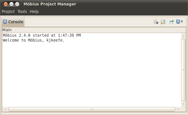
Contents

Project Manager[edit]

The Project Manager is the main console for Möbius and is shown in <xr id="fig:projman" />. Across the top is a main menu, with three menu categories: Project, Tools, and Help. The main display is a console view that shows messages for the operations performed by Möbius. Descriptions of the operations available under each menu category are presented in the following sections.


<figure id="fig:projman">

Projman.png


<xr id="fig:projman" nolink />: The Project Manager window.
</figure>


Project Menu[edit]

The Project menu contains several operations related to Möbius projects. A Möbius project is the fundamental unit of organization for each system model in Möbius. A project contains one or more models defining the system and instances, descriptions of what parameters to solve for, and instances of solvers to generate the solutions. More details on projects can be found in Section 2.

The Project menu contains the following operations:

  • New: Create a new project. A dialog will appear prompting for the new project name. After you enter a valid project name, the author, and a description. The author and description are optional and for informational purposes only. These two fields can be changed at a later date. The new project will be opened.
  • Open: Open an existing project. A dialog to select the project to open will appear as shown in <xr id="fig:project_dialog" />. You may select multiple projects to be opened simultaneously. You can quickly open a single project by double clicking it.


<figure id="fig:project_dialog">

Projman projdialog.png


<xr id="fig:project_dialog" nolink />: Use the project selection dialog to open projects.
</figure>


  • Copy: Copy an existing project to a new project. You must close the existing project to guarantee a stable copy.
  • Rename: Give an existing project a new name. You must close the project before it can be renamed.
  • Clean: Remove all temporary files from the project.
  • Resave: Regenerate all project source code and libraries. Resaving the project is required before a project is opened for the first time after a Möbius upgrade. You must also resave after unarchiving a project.
  • Delete: Delete the project. The most-recently-deleted project is stored in a “Deleted” folder within the Möbius project directory.
  • Archive: Create a backup of the project. After you select one or more projects, you will be asked for details about how you want each of the selected projects to be archived. After you specify the name of the archive file, you must select one of two options, Full archive and Minimal archive. A full archive includes all files found within the project. A minimal archive includes only the files necessary to define all models within the project. In a minimal archive, object files, libraries, executables, and results are not backed up. Minimal archives are helpful when multiple users are collaborating on the same model, since they create small archives that are convenient to email. The format for the archive is gzipped tar (.tgz) format.
  • Unarchive: Restore a project from an archive file. If the project to be restored has the same name as an existing project, you can either delete the existing project or cancel the restoration. Restoring one project on top of a different one could cause corruption and confusion, so is not supported. Unarchived projects should be resaved before they are used.
  • Document: Create HTML documentation for the chosen project. After you select the project to document, you use the Document Project dialog (see <xr id="fig:doc_proj" />) to select the models in the project that should be documented. Documentation is written to a subdirectory in the Documentation directory within the selected project’s project directory. The name of the subdirectory is given by the Document Name field in the dialog. You can view it with a web browser, or import it into software such as Microsoft Word for format refinement and printing.
Möbius supports three image formats for output: PNG, SVG, and PDF. You select which formats you want generated by selecting the appropriate checkboxes. Also, you can include one of these outputs into the generated HTML documentation.
There are four options in the dialog that are helpful when dealing with images that are too large to fit on a single page:
Generate one complete image will create a single image for the model.
Generate subimages if necessary will subdivide the full image in width and/or height and generate two or four subimages. The width is subdivided if the original image is more than 650 pixels wide. The height is subdivided if the original image is more than 700 pixels tall.
Scale subimages will scale each subimage that is larger than a single page in size. The scaling is proportional and the resulting image will be at most 650 wide or 700 pixels tall.


<figure id="fig:doc_proj">

Projman document.png


<xr id="fig:doc_proj" nolink />: The Document Project dialog is used to select models from the project to include in the documentation.
</figure>


  • Preferences: Launch the preferences window (see <xr id="fig:projman_preferences" />).


<figure id="fig:projman_preferences">

Projman preferences.svg


<xr id="fig:projman_preferences" nolink />: The Möbius Preferences dialog is used to change various preferences about the operation of Möbius.
</figure>


  • Quit: Exit Möbius.

Preferences Dialog[edit]

The Preferences dialog (<xr id="fig:projman_preferences" />) provides access to various preferences and settings used during the operation of the Möbius tool. The preferences are broken down into pages listed on the left side of the dialog. Above the pages is a filter text box that you can quickly type a keyword in and the preference pages pertinent to that keyword will be displayed. For example, typing “user” in the filter box will eliminate all the pages except the Database page, because it contains a username field used by the database connection feature.

The Preferences dialog contains the following page:

  • Build: This preference page allows you to define the default compile mode and default simulation execution architecture. Möbius can compile in two modes: normal and optimized. Normal mode incorporates compiler-created debugging symbols into the object files, and uses debug-enabled Möbius AFI libraries when creating the executables, allowing project-generated executables (such as the simulator and state-space generator) to be run through C++ debuggers like gdb. Normal mode also enables Möbius trace output, making it possible to generate files that trace the progress of the model during solution. Normal mode object code takes less time to generate, but is often much larger than optimized code, due to the extra debugging symbols that are included.
Optimized mode enables full compiler optimizations, and disables debug symbols and trace output. Optimized mode should be used when the model is running well, and results need to be produced rapidly.
The results generated should be the same in either mode. The modes allow for the trade-off between extra information needed for debugging and speed of data production.
The default simulation execution architecture mode has two options: 32-bit and 64-bit. For machines running a 32-bit version of their operating system, this setting has no effect as simulations will always be executed in 32-bit mode. However, for machines running a 64-bit operating system, you have the option of building and executing 32-bit or 64-bit simulations. 32-bit simulations will likely run a little faster and take up significantly less memory during execution. However, 64-bit simulations enable access to greater amounts of memory space that may be necessary for large simulations. Simulation results in either mode should be the same.
  • Database: The Database settings dialog displays the list settings that are needed to interface Möbius the integrated results database features with the external database server.


<figure id="fig:projman_db">

Projman database.png


<xr id="fig:projman_db" nolink />: The Results Database preference page is used to specify the database access settings.
</figure>


Database Enabled determines if Möbius will connect to the database server using the specified configuration settings.
User Name specifies the name of the database user that Möbius should use when connecting to the database system.
Password specifies the password for the indicated database user.
Database is the name of the database Möbius will create. Multiple databases can be created as needed, simply by changing this name.
Hostname is the name of the machine where the database server is located. Can be a full machine name or “localhost”.
Port is the listening port of the database server. The default port is 5432. Ask your system administrator if the port was changed when the database server was configured.
  • External Tools: The External Tools preference page lists the external tools Möbius uses during its operation. In special cases, you may want to change the tool used to perform a certain operation (for example, the remote shell or archive command). The provided tool must either be in your PATH or the absolute path to the tool should be provided. Some fields are used to specify additional arguments to the external tool whenever it is called.
Compiler: The G++ compiler that Möbius should use.
Compiler Options: Extra compiler options to be used when compiling the Möbius project. This field was originally used to add debugging flags. In current versions, debugging flags are automatically added as part of the normal compilation mode, and this field should typically be blank.
Linker: The linker, ld. Usually set to the path to the standard linker for the system.
Linker Options: Extra linker options to be used when linking Möbius solvers (such as the simulator and state-space generator). For standard use, this field can be left blank.
Make Command: The GNU make tool. The version of make should be 3.7x or later.
Archive Command: The ar tool, the system command used to create C++ library files.
Ranlib Command: The ranlib tool. Ranlib is used during the creation of project libraries.
Remote Shell Command: The command used to gain remote access to other machines on the network. It is not necessary to specify a remote shell command to run Möbius on a single local machine. Typically this command is either rsh or ssh. In either case, system access privileges must be set so that the command can execute without entering a password or pass phrase. More details are available in Appendix section ?? and in the system man pages for rsh and ssh.
Tar Command: The GNU tar command. This command is used to create and restore archive files. NOTE: In the current version of Möbius, tar is used with the “z” option, specifying the archive to be compressed with gzip. Typically gzip is installed in the same directory as tar, but most implementations of tar expect to find gzip in the PATH, and do not expect to have to look for it. If there are error messages when “archive” or “unarchive” commands are run, please see if gzip is found in the system PATH, and update the PATH if necessary.
  • Locations: The locations preference page contains a list of system paths necessary for the operation of Möbius.
Möbius Installation Path: The directory where the Möbius software is installed. This field should update automatically, based on the location of the Möbius executable currently running. Möbius uses this directory to locate the Möbius AFI header files and libraries.
Möbius Projects Directory: The directory containing the desired set of Möbius projects. It is possible to have multiple project directories, and changing this field switches from one to another. Most new users find one project directory is sufficient. The project path should not contain spaces. As a result, the default path on Windows is C:MobiusProject. If multiple people are using Möbius on the same machine, they should all give unique names for their Project directories.


Tools Menu[edit]

The Tools menu lists the various utilities available in Möbius. The Data Manager menu item will launch the Möbius Data Manager, which is further described in Section 1 of Utilities.


Help Menu[edit]

The Help menu provides various help for the use of Möbius. The About menu item opens the About window. The About window contains information about this version of Möbius, including the vendor and copyright statement.


Console View[edit]

The Console View provides a running output of the operations of Möbius. When a project is opened or a model component is saved, this event is logged by the console for your review. The Console View has several icons in the upper right corner to control the behavior of the console and to switch between the available console logs.

The first icon looks like a document with a grey X over it. This icon clears all the text from the current console log. This can be useful for when you want a fresh start to the log.

The next icon has a lock over a scrolling control. This is the scroll lock and will prevent the console from autumatically scrolling down as new text is appended to the console.

The next icon has pin on a window icon. This is the pin console button and will keep the console view from switching to a different console automatically.

Finally, the last icon allows you to switch between the available console logs. The Main console provides general information about the operation of Möbius. The Error console provides detailed error messages when something goes wrong. The Detailed console provides the finest grain of detail messages possible and includes messages from the other two consoles. Of particular interest, when Möbius executes an external command (e.g. make, java, etc.) the command and its arguments are logged in the Detailed console.

The text of a console log can be highlighted for copy/paste operations like you would expect. Also, if you right click on the text, a simple find feature is available to quickly search through the contents of the log.


Project Editor[edit]

The Möbius project is the fundamental unit of organization for each system model in Möbius. A complete project will contain the following: one or more models defining the system behavior, a description of what to measure about the system, specification of all model parameters, at least one instantiation of a solver to compute the required measurements, and the results produced by the solver.


Tree View[edit]

The model types in the project are classified in the same hierarchy as the components of the Möbius framework (see section 1 of Modeling Background). The model types that may exist in a project are listed below.

  • Atomic models describe the behavior of individual components of the system.
  • Composed models are hierarchical models used to combine atomic and composed models to form the complete model of the system.
  • Reward models define measures of interest about the system.
  • Study models create experiments that specify values for the system parameters in the model.
  • Solvers solve the model using simulation, or prepare the model for numerical solution using state-space generation.
  • Numerical solvers solve the model using a variety of numerical algorithms.

The model types are arranged in a tree, in which the names of the various classifications are the main nodes, and the instances of each classification are the children of the node. The tree view from an example project editor is shown in <xr id="fig:project_main" />.


<figure id="fig:project_main">

Project main.png


<xr id="fig:project_main" nolink />: Tree view in the project editor, with Atomic selected.
</figure>


The order of model types in the tree represents the typical dependency among models in a project. A model of a given type typically depends on models of the type one level above it in the tree. For example, a study model depends on a reward model. When one model depends on another, it is often referred to as the parent, and the model it depends on is referred to as the child.


Project Operations[edit]

Several operations are possible in the project editor. You can access the operations via the toolbar or through a pop-up menu activated by right-clicking within the tree view.


New     To create a new model within a project, select the desired category and click on New. A dialog will appear, asking for the type of formalism to create. For example, <xr id="fig:model_creation#1" /> displays the possible types of atomic models that can be created. The dialog also gives the opportunity to name the new model.

After you click the OK button, the new model editor will open. In the case of the reward, study, solver, and numerical solver models, another pop-up dialog will immediately appear, requesting the name of the child model of the new model, as shown in <xr id="fig:model_creation#2" />.

<figure id="fig:model_creation">

<subfigure>Project atomic.png</subfigure> <subfigure>Project child.png</subfigure>
(a) Specify the name and type of newly created models. (b) Specify the newly created model’s child model.
</figure>
<xr id="fig:model_creation" nolink />: Dialogs shown when a new Möbius model is created.


Open     Select a model name from the tree view, and then click Open to open it. Multiple models may be open at the same time.


Copy     Select a model name or type from the tree view, and then click Copy to generate a copy of the model. Another dialog opens, allowing you to copy the selected model to another file within this project, or copy it into another project. Also, you can copy models from another project into the current one.


<figure id="fig:project_copy">

Project copy.png


<xr id="fig:project_copy" nolink />: An instance of the copy dialog, which is used to copy models within a project, or from one project to another.
</figure>


Import     Select a model type in the tree view and then click Import to import this type of model from an existing UltraSAN1 project. A dialog will appear, listing all the UltraSAN projects found in the UltraSAN project directory (see Section ?? on how to set the UltraSAN project directory). After you select one of the UltraSAN projects, another dialog will appear listing all possible models in the UltraSAN project of the type selected in Möbius.

1 UltraSAN was the predecessor to Möbius.


Delete     You can delete a model in a Möbius project by selecting the model in the tree view and choosing the Delete menu.


Close     You can close the project editor using the Close button, after all of the model editors of the project have been closed.


Project Directory Structure[edit]

Each project is stored in a directory named after the project within the Möbius project directory. It is necessary to understand the basic structure of a project directory, since Möbius stores output files, such as solution results or model documentation, in various locations within the project subtree. Files within the project directory are arranged in the same tree structure as the tree view.

Solution results and other solver outputs are typically written to the model directory corresponding to the solver that generated the results.

All documentation is stored in a subdirectory of the Documentation directory in the top-level directory of the project. The name of this subdirectory is given by the Document Name field in the Document Project dialog. See <xr id="fig:doc_proj" /> for an example.

The project and each model in the project are defined in separate files, which are also named after the project or individual model and have extensions unique to each type of model. The files are XML-based, and under most circumstances should not be edited directly. Doing so can corrupt the Möbius project.


Constraints Checker[edit]

When a project, or a submodel within the project, is saved in the Project Editor, the constraints checker is called by the Project Manager to ensure that the model, as saved, doesn’t violate any conditions imposed upon it by solver modules which utilize the model. If the constraints checker detects a violation of a constraint, it produces a pop-up warning informing the user of the problem, prompting them to correct the issue.

For more on specific constraints for individual solvers, see section 4 of Solving Models.


Model Editors[edit]

Common Menus[edit]

There are several menus that are common to each model editor in Möbius. Instead of describing these features repeatedly, the functionality common to each model editor is discussed in this section.

File[edit]

The File menu is common to all editors, and typically contains the following common commands:

  • Save: Store the current model to disk, and then translate the model into the appropriate C++ code and compile the code to form the representative library for this model.
  • Save No Compile: Store the current model to disk, but avoid performing the compilation. It is still necessary to compile the model, either by selecting Save from the File menu, or by compiling within the solver.
  • Close: Close the editor. If there are unsaved changes, a dialog will appear, prompting you to save before closing.
  • Document Model: Create HTML documentation for the current model. The documentation files will be stored in a subdirectory in the Documentation directory within the project’s project directory. The name of the subdirectory will be what you specify in the Document Name field of the dialog box. See <xr id="fig:doc_proj" />.

Edit[edit]

Undo

You are allowed to undo most recent operations on the model using the Undo menu. Examples of operations that can be revoked using the undo feature include the movement of graphical components in an editor, the renaming of components, the editing of text, the addition of new components, and the addition of lines. The Undo menu will list the name of the most recently completed operation that can be undone. Undo operations are stored so that multiple operations can be undone.


Edit global variables

The behavior of complex systems being modeled often depends on several parameters. Often these parameters are unknown, or can take on multiple values, depending on the configuration of the system. Möbius provides the option of using global variables instead of pure numerical values to define the different characteristics of elements like state variables and actions. The values of the global variables are then set by experiments in the study model.

In each atomic or composed model, you can add or delete global variables by clicking on the Edit Global Variables option on the menu editor. A pop-up dialog box, as shown in <xr id="fig:atomic_san_editor_global_variables" />, is used to add, delete, and view global variables. The dialog box can remain open as a reference while you are editing the model.


<figure id="fig:atomic_san_editor_global_variables">

Atomic san editor global variables.png


<xr id="fig:atomic_san_editor_global_variables" nolink />: Global Variables editor.
</figure>


  • The Add button is used to create new global variables. The combo-box on the top-right corner lists the available data types for the global variable. Only the standard data types that C++ directly supports are currently allowed (char, double, int, long, float, and short).
  • The Delete button is used to delete the selected global variables.
  • The Close button is used to hide the Global Variables editor dialog box.


User-defined functions

While building models, you might find it useful to define functions for the model using C++ header files and libraries. These functions are stored in C++ header (.h) or possibly source (.cpp) files that you must create. The files can be placed anywhere, but most often are stored in a new subdirectory in the project. If you are using C++ source files (.cpp), you will also need to place into the same directory a Makefile that will compile the source files into a library. The simplest way to create the Makefile is to copy one from an atomic model in your project and modify it to compile the library. With the current version of Möbius, you must compile the library manually before running a solver. Otherwise, an error message stating the library is missing will appear when the compiler tries to link with the user-defined library in the solver.

After you have successfully compiled the source code and created the library, you need to let Möbius know the location of the functions. You can do this by opening any model and selecting User-Defined Header under the Edit menu. A dialog box will pop up, asking for the location of your header (see <xr id="fig:atomic_san_editor_user_defined_header" />).


<figure id="fig:atomic_san_editor_user_defined_header">

Atomic san editor user defined header.png


<xr id="fig:atomic_san_editor_user_defined_header" nolink />: User-defined header editor.
</figure>


Enter the path to the C++ header file. There is a check box that instructs Möbius to store the header file path relative to your Möbius project directory. You should check it if your header files are stored in a subdirectory of your project, as it makes it easier to share your project with other users, or relocate it to different systems. If the path entered is incorrect, or the file has not yet been created, Möbius will display an error message.


<figure id="fig:atomic_san_editor_user_defined_library">

Atomic san editor user defined library.png


<xr id="fig:atomic_san_editor_user_defined_library" nolink />: User-defined library editor.
</figure>


If you are also using a user-defined library, repeat the same operation for the library (see <xr id="fig:atomic_san_editor_user_defined_library" />). This dialog contains the same relative path checkbox found in the User-Defined Header dialog. It also contains another checkbox that makes it possible to support multiple operating system versions of the user-defined library. This feature will only work if the library name contains the name of the current operating system: Solaris, Linux, or Windows. After you check this box, the operating system name is replaced with $ARCH. When Möbius compiles your project on each operating system, $ARCH is replaced with the name of the appropriate operating system.

User-defined functions can be extremely useful if you are trying to make models more modular, or if multiple elements, such as SAN output gates, within the model are performing similar operations. In fact, you can even define functions that would modify the values of elements within the model (for example, a place within a SAN). Here are a few examples in which user-defined functions are helpful:

  • If your model contains complex functions that are repeatedly used or susceptible to change, you can write them in the library and simply call them from the model. For example, to define a comparison between two extended places that are arrays of 2 integers, you can create the following function in the library:
inline int is_lower(int x1, int y1,
int x2, int y2) {
if (x1<x2) return 1;
else if (x1 == x2) {
if (y1 <= y2) return 1;
else return 0;
}
else return 0;
}
The following code shows how to use the function in the model:
short result = is_lower(Place1->x, Place1->y,
Place2->x, Place2->y);
if (result == 1)
...
  • In the same way, you can define enabling conditions for activities using user-defined functions:
inline int activity_enable(int value1,
int value2) {
int ret=0;
if (value1==0 && value2==0)
ret=1;
...
return ret;
}
The enabling function of the corresponding input gate would then call the user-defined function, as follows:
activity_enable(Command1->Mark(),
Command2->Mark(), Group_ID->Mark(),
Component_ID->Mark(),
Component_type->Mark())
  • If you have an extended place in your model with a type that is a large array, matrix, or structure, it is possible to write a user-defined function to initialize the extended place. If you want to create unique experiments that define different initial values for this extended place, you can create a single global variable, and then write the user-defined function so that the extended place is initialized with different values, based on the value of the global variable. Then in the study you only need to adjust one value to change the definition of all fields in the extended place.


Atomic Formalisms[edit]

Each model is composed of one or more submodels, also referred to as atomic models. You can create and edit atomic models using different editors like the SAN editor, the PEPA editor, the Buckets and Balls editor, and the Fault Tree editor.


ADVISE[edit]

Mobius supports multiple modeling formalisms, including ADversary VIew Security Evaluation (ADVISE). ADVISE allows modelers to create and analyze a specific adversary profile in an executable state-based security model of a system (11LEM02). Using graphical primitives, ADVISE provides a high-level modeling formalism to easily create the adversary profile and the executable state-based security model of the system under consideration.

ADVISE Primitives[edit]

ADVISE models consist of five primitive objects: attack steps, accesses, knowledges, skills, and goals. Attack steps represent the actions taken by the adversary. Accesses, knowleges, and skills represent the accesses, knowledge, and skills of the adversary, respectively. Goals represent the goals (or flags) of the adversary.

Attack Step[edit]

Attack steps represent the actions taken by the adversary. Attack steps are represented graphically as rectangles. An attack step is fully described by its input, output, and properties. An attack step can have inputs from accesses, knowledges, skills, and goals. It can also have outputs to the same four types of elements (accesses, knowledges, skills, and goals). An attack step also contain four properties: attack cost, attack evaluation time, preconditions, and outcomes.

The attack cost of an attack step represents the relative cost of the attack step with respect to the adversary. For example, if an attack step is difficult or expensive (such as hacking into a locked vault door), then the attack cost will be relatively large. If the attack step is easy or inexpensive (such as opening an unlocked door), then the attack cost will be relatively small. Since an adversary is more likely to take the easiest route to the goal, she will likely choose an attack step with a lower attack cost over one with a higher attack cost.

The attack execution time of an attack step represents the relative time it will take to complete the attack step. For example, if an attack step will take a long time to complete (such as downloading several terabytes of logs), then the attack execution time will be relatively large. If the attack step will not take much time to complete (such as downloading a few kilobytes of a small subset of the logs), then the attack execution time will be relatively small. Since an adversary is more likely to take the quickest route to the goal, she will likely choose an attack step with a shorter attack execution time over one with a longer attack execution time.

The preconditions of an attack step represent the conditions that must take place before the adversary is able to attempt the attack step. The preconditions of an attack step are closely related to the inputs of the attack step since the inputs of the attack step provide the state variables of the model that can be used in the conditional expression. For example, if the attack step requires a certain access and level of skill to attempt, then the inputs of the attack step would be that access and that skill, and the precondition of the attack step would be a conditional expression such as \verb|return (access1 && (skill1 > 0.7)|. As a more concrete example, suppose the attack step is to pick the lock on a safe. The access in this case would be having close proximity to the lock, and the skill would be lock-picking.

The outcomes of an attack step represent the outcomes that occur if the attack step is successfully completed. The outcomes of an attack step are closely related to the outputs of the attack step since the outputs of the attack step provide the state variables of the model that can be modified depending on the resulting outcome. Every attack step has one or more outcomes, each with a probability of occurring. The sum of the probability of each of the outcomes of the attack step is always 1. Each outcome also has an associated detection probability which represents the probability that the adversary will be detected if this outcome occurs. Since an adversary is likely to want to avoid being detected, she will likely choose attack steps with a lower weighted detection probability of its outcomes over an attack step with a higher weighted detection probability of its outcomes.

Access[edit]

Accesses represent the relevant accesses the adversary may have (or eventually gain) in the executable state-based security model of the system. Accesses are state variables that store whether or not the adversary has the given access. An access may represent a physical access (such as close proximity to a target or having a key to a relevant door in the model) or a more abstract access (such as administrator privileges in a target machine). Accesses are represented graphically as purple squares.

Knowledge[edit]

Knowledges represent the relevant knowledge the adversary may have (or eventually gain) in the executable state-based security model of the system. Knowledges are state variables that store whether or not the adversary has knowledge of the given information. Knowledge may represent a fact such as the adversary knowing a certain password of a target system or the type of encryption that is used between two target nodes. Knowledges are represented graphically as green circles.

Skill[edit]

Skills represent the relevant skills the adversary may have (or sometimes may eventually gain) in the executable state-based security model of the system. Skills are state variables that store the extent to which the adversary is skilled in that given area. For example, a certain adversary may have a lock-picking skill of 0.7 which could mean that she is adept at lock-picking, but not yet a master of the skill. Skills are represented graphically as blue triangles.

Goal[edit]

Goals (or flags) represent what the adversary is trying to ultimately achieve. Goals are state variables that indicate whether or not the adversary has accomplished the goal yet. Goals can represent achievements such as successfully accessing sensitive information, shutting down a target system, or escaping from a bank with stolen jewels. Goals are represented graphically as gold ovals.

Editor[edit]

This section looks into the atomic formalism that represents ADVISE with emphasis on creation, editing, and manipulation of atomic models using the Mobius ADVISE editor.

TODO - Finish this section

Edit[edit]

TODO - finish this section

View[edit]

TODO - finish this section

Elements[edit]

Elements are ADVISE model primitives. The Elements menu includes the following types of elements:

  • Attack step - rectangle
  • Access - purple square
  • Knowledge - green circle
  • Skill - blue triangle
  • Goal - gold oval

TODO - finish this section

SAN[edit]

Möbius supports multiple formalisms, including stochastic activity networks (SANs). SANs[1] are stochastic extensions to Petri nets[2]. Using graphical primitives, SANs provide a high-level modeling formalism with which detailed performance, dependability, and performability models can be specified relatively easily.

SAN primitives[edit]

SANs consist of four primitive objects: places, activities, input gates, and output gates. Activities represent actions of the modeled system. Places represent the state of the modeled system. Input gates are used to control the “enabling” of activities, and output gates are used to change the state of the system when an activity “completes.”


Places     Places represent the state of the modeled system. They are represented graphically as circles. In <xr id="fig:atomic_san_editor" />, memory_chips, interface_chips, memory_failed, and computer_failed are places. Each place contains a certain number of tokens, which represents the marking of the place. The set of all place markings represents the marking of the stochastic activity network. Note that tokens in a place are homogeneous, in that only the number of tokens in a place is known; there is no identification of different kinds of tokens within a place.


<figure id="fig:atomic_san_editor">

Atomic san editor.png


<xr id="fig:atomic_san_editor" nolink />: Möbius SAN Editor.
</figure>


The meaning of the marking of a place is arbitrary. For example, the number of tokens in a place could represent a number of objects, such as a number of tasks awaiting service. Also, the number of tokens in a place could represent an object of a certain type, such as a task with a certain priority level. This dual nature of a place marking provides a great deal of flexibility in modeling the dynamics of a system.


Activities     Activities represent actions in the modeled system that take some specified amount of time to complete. They are of two types: timed and instantaneous. Timed activities have durations that impact the performance of the modeled system, such as a packet transmission time or the time associated with a retransmission timer. Timed activities are represented graphically as thick vertical lines. In <xr id="fig:atomic_san_editor" />, memory_chip_failure and interface_chip_failure are timed activities. Each timed activity has an activity time distribution function associated with its duration. Activity time distribution functions can be generally distributed random variables. Each distribution can depend on the marking of the network. For example, one distribution parameter could be a constant multiplied by the marking of a certain place. Instantaneous activities represent actions that complete immediately when enabled in the system. They are represented graphically as thin vertical lines. No instantaneous activities are represented in <xr id="fig:atomic_san_editor" />. Case probabilities, represented graphically as circles on the right side of an activity, model uncertainty associated with the completion of an activity. Each case stands for a possible outcome, such as a routing choice in a network, or a failure mode in a faulty system. In <xr id="fig:atomic_san_editor" />, activity interface_chip_failure has three cases. Each activity has a probability distribution, called the case distribution, associated with its cases. This distribution can depend on the marking of the network at the moment of completion of an activity. If no circles are shown on an activity, one case is assumed with a probability of one.

An activity is enabled when the predictes of all input gates connected to the activity are true, and all places connected to incoming arcs contain tokens, i.e. have non zero markings. Once enabled, the activity samples its delay distribution function to determine the time delay before the activity fires. When the activity fires it updates the state of the model by subtracting tokens from places connected by incoming arcs, adding tokens to places connected by outgoing arcs, and executing the functions in input and output gates. The specific order that the state updates occur is: input gates, input arcs, output gates, and finally output arcs.

Please be aware that the order in which state updates occur in Möbius differs from UltraSAN. Gates are executed before arcs in Möbius, but the opposite was true in UltraSAN. Also, if there are multiple instances of the same item, for instance multiple input gates, the order of application of the gates is not specified. Models must be constructed so that the gate functions are execution order independent any time there are multiple instances of the same type of gates connected to an activity.

Also associated with each activity is a reactivation function. This function gives marking dependent conditions under which an activity is reactivated. Reactivation of an activated activity means that the activity is aborted and that a new activity time is immediately obtained from the activity time distribution. The reactivation function consists of an activation predicate and a reactivation predicate. An activity will be reactivated at the moment of a marking change if (1) the reactivation predicate holds for the new marking, (2) the activity remains enabled, and (3) the activation predicate holds for the marking in which the activity was originally activated.


Input gates     Input gates control the enabling of activities and define the marking changes that will occur when an activity completes. They are represented graphically as triangles. In <xr id="fig:atomic_san_editor" />, IG1 and IG2 are input gates. On the other side of the triangle is a set of arcs to the places upon which the gate depends, also called input places. Each input gate is defined with an enabling predicate and a function. The enabling predicate is a Boolean function that controls whether the connected activity is enabled. It can be any function of the markings of the input places. The input gate function defines the marking changes that occur when the activity completes.

If a place is directly connected to an activity with an arc, it is equivalent to an input gate with a predicate that enables the activity whenever the place has more than zero tokens along with a function that decrements the marking of the place whenever the activity fires.


Output gates     Like input gates, output gates define the marking changes that will occur when activities complete. The only difference is that an output gate is associated with a single case. An output gate is represented graphically as a triangle with its flat side connected to an activity or a case. In <xr id="fig:atomic_san_editor" />, OG1, OG2,..., OG6, and OG7 are output gates. On the other side of the triangle is a set of arcs to the places affected by the marking changes. An output gate is defined only with a function. The function defines the marking changes that occur when the activity completes. There is also a default scenario for output gates. If an activity is directly connected to a place, it is equivalent to an activation in which an output gate has a function that increments the marking of the place whenever the activity is fired.

More information on SANs can be found in [1]. The next few sections describe the various features available in the SAN editor to develop a SAN model.

Editor[edit]

This section looks into the atomic formalism that represents stochastic activity networks with emphasis on creation, editing, and manipulation of atomic models using the Möbius SAN editor. Refer to Section 2 for details on how to create and open a SAN model.

The names of the selected project and subnet appear in the top left corner (see <xr id="fig:atomic_san_editor" />). The large gridded area in the center is the drawing area . In the case of a new model, this gridded area is blank. Like most applications, the editor lists the menu horizontally at the top of the application’s current active window. If you click on a menu item, it drops a tool panel containing several options. The menu items and tool panel options are used to create and draw in the SAN formalism, as discussed below.

As discussed in Section 3.1, many menus are common to all model editors within Möbius. Please see Section 3.1 for detailed descriptions of the common editor functions. The following paragraphs will discuss the functionality that is unique to the SAN editor.

Edit[edit]

Type definitions

The SAN formalism supports a special element called extended place that allows the model to handle the representation of structures and arrays of primitive data-types. Clicking on Type Editor opens the dialog box shown in <xr id="fig:atomic_san_editor_user_type_definition" />. In this dialog box, you can create new structures and arrays that can be associated with extended places.


<figure id="fig:atomic_san_editor_user_type_definition">

Atomic san editor user type definition.png


<xr id="fig:atomic_san_editor_user_type_definition" nolink />: SAN user-type definition editor.
</figure>


  • Use the Edit button to edit any currently defined user-defined types. The GUI can automatically tell if the user is editing an array (see <xr id="fig:atomic_san_editor_user_type_definition_array" />) or structure (see <xr id="fig:atomic_san_editor_user_type_definition_structure" />) and appropriately open the required editor. You are expected to click on the available list of user-defined types to edit them. The editor allows you to change the name of any user-defined type, even if the user-defined type is declared as a field in another user-defined type or associated with an extended place. The interface takes care of updating all the changes.
  • Use the Delete button to delete the selected user-defined type that is not being used by any other user-defined type and is not associated with any extended place. If you attempt to delete a type that is in use, an error dialog box pops up. A successful delete removes the user-defined type from the current list.
  • Use the New Struct button to pop up a new dialog box that allows you to create a new structure-type definition. The pop-up dialog box layout is depicted in <xr id="fig:atomic_san_editor_user_type_definition_structure" />.


<figure id="fig:atomic_san_editor_user_type_definition_structure">

Atomic san editor user type definition struct.png


<xr id="fig:atomic_san_editor_user_type_definition_structure" nolink />: SAN struct-type definition editor.
</figure>


– Use the Name text box to define a name for the structure.
– The Fields list shows the fields you declared in the current structure.
– The New field button adds a new field to the structure. The combo-box on the left lets you choose the type of the field from a list of the standard data types and user-defined data types. Recursive definitions or pointers are not allowed.
– The Delete button deletes the selected field.
– The Move up button moves the selected field up by one position.
– The Move down button moves the selected field down by one position.
– The OK button accepts all changes made and hides this dialog box, bringing the User-type definitions editor to the front. An error message pops up you try to create a structure with no fields or a structure that has no name or a non-unique name.
– The Cancel button discards all changes, hides this dialog box and returns you to the User-type definitions editor.
  • The New Array button pops up a new dialog box that allows you to create a new array-type definition. The pop-up dialog box layout is depicted in <xr id="fig:atomic_san_editor_user_type_definition_array" />.


<figure id="fig:atomic_san_editor_user_type_definition_array">

Atomic san editor user type definition array.png


<xr id="fig:atomic_san_editor_user_type_definition_array" nolink />: SAN array-type definition editor.
</figure>


– The Name text box allows you to define a name for the array.
– The Definition combo-box allows you to select the data type for the array. The choices include primitive data types or user-defined types. You are also expected to declare the size of the array. The elements of the array are generically labeled as index.
– The Initialize all array elements to common value checkbox makes it easier to manage large arrays. If it is known when the array type is defined that all elements in the array should be initialized to the same value, 0 for instance, clicking this box will avoid the need to initialize each element separately. This option is critical when defining very large arrays because it saves a significant amount of memory within the Möbius editor process.
– The OK button accepts all changes made, hides this dialog box, and returns you to the User-type definition editor. An error message will pop up if you try to create an array with an invalid size (i.e., a non-numeric, zero, or negative size) or an array that has no name or a non-unique name.
– The Cancel button discards all changes, hides this dialog box, and brings you back to the User-type definition editor.
  • The OK button hides the User type definitions dialog box and brings you back to the SAN editor.

View[edit]

Increase size and Decrease size

Click on menu item Increase Size to increase the size of the drawing area. Click on Decrease Size to decrease the size until the scroll bar disappears or becomes equal to area on which the model elements are spread. You can increase the size of the drawing area, scroll down to the extra space created, and add new components to the model, if necessary.


Zoom in and Zoom out

Each time you click on the menu item Zoom In, the GUI enlarges the drawing area by a fixed percentage. The interface takes care of adding scroll bars if necessary so that the entire model can be viewed. To keep the model in focus, be careful not to multiple-click on this option. Zoom Out decreases the size of the model until the scroll bars disappear.


Grid setting

Click on the menu item Grid Setting to open a dialog box as shown in <xr id="fig:atomic_san_editor_grid_setting" />. Here, you can define the X and Y coordinate size of the grid in pixels. Note that if you set the grid to 1 pixel size, it will take an extremely long time to render the model. You can adjust the grid according to your comfort level. There are a few checkboxes on the Grid Setting dialog box. They are Enable display grid points, Enable snap to grid for object placement, and Snap existing objects to grid. Each checkbox is self-explanatory. Use the OK button to accept the changes or the Cancel button to discard the changes. Either way the dialog box will close so that you are returned to the SAN Editor.


<figure id="fig:atomic_san_editor_grid_setting">

Atomic san editor grid setting.png


<xr id="fig:atomic_san_editor_grid_setting" nolink />: SAN user Grid Setting Dialog editor.
</figure>


Elements[edit]

Elements are SAN model primitives. The Elements menu includes the following types of elements:

  • Place, which will be represented by a blue circle.
  • Extended Place, which will be represented by an orange circle.
  • Input Gate, which will be represented by a triangle with its tip pointing to the left.
  • Output Gate, which will be represented by a triangle with its tip pointing to the right.
  • Instantaneous Activity, which will be represented by a solid vertical bar. If the activity has multiple cases, they appear as small circles on the right side of the vertical bar.
  • Timed Activity, which will be represented by a hollow vertical bar. It has small circles on its right side if it has multiple cases.

You can also select a SAN model element by clicking the left button on the required component while the cursor is on the menu item Elements. SAN elements can also be accessed via icons below the menu. To place one of those components, click on it, move it to the desired location, and place it by clicking the left mouse button. A dialog box will appear asking you to specify various attributes relevant to the element type. The name must be unique across the current atomic model. The name also must follow the C++ variable naming convention. The rest of this section discusses various parameters of each model element.


Place

When you create or edit a place (by right-clicking on the place and clicking on Edit in the pop-up window), a dialog box similar to the one shown in <xr id="fig:atomic_san_editor_place_attribute" /> appears.


<figure id="fig:atomic_san_editor_place_attribute">

Atomic san editor place attributes.png


<xr id="fig:atomic_san_editor_place_attribute" nolink />: Place Attributes dialog box.
</figure>


  • The Name text box allows you to modify the name, provided that the new name is unique in the current model.
  • The Token(s) text box allows you to edit or modify the initial marking. The value should be a non-negative short integer, which implies that place markings can only be non-negative integers less than or equal to 32,767. However, the initial marking may be defined as a scalar value, or as a global variable. The following points about global initial marking must be noted:
– global variables for places must be of type short.
– global variables for initial markings should not be arithmetic expressions, or functions of other initial global markings.
  • The OK button accepts the changes and returns you to the SAN Editor. It pops up an error message if there is a problem in validating the tokens text box.
  • The Cancel button discards the changes and brings you back to the SAN Editor.


Extended place

When you create or edit an extended place (by right-clicking on an extended place and clicking on Edit in the pop-up window), a dialog box similar to that shown in <xr id="fig:atomic_san_editor_extended_place_attribute" /> appears.


<figure id="fig:atomic_san_editor_extended_place_attribute">

Atomic san editor extendedplace attributes.png


<xr id="fig:atomic_san_editor_extended_place_attribute" nolink />: Extended Place Attributes dialog box.
</figure>


  • The Name text box allows you to modify the name provided that the new name is unique in the current model.
  • The Initial value tree represents the current values associated with the structure or array of the extended place. Only the leaf nodes can be initialized to a particular initial value. Clicking on intermediate nodes hides the visible text box. Each time you click on a new leaf node, the GUI evaluates the current initial value for validity, displaying error messages if necessary.
  • The text box allows you to edit/modify the initial marking(s) of the selected leaf nodes of the structure or an array. However, the initial marking may be defined as a scalar value, or as a global variable. The following points about global initial marking should be noted:
– global variables for extended places must be of the same type as the corresponding leaf field.
– global variables for initial markings should not be arithmetic expressions, or functions of other initial global markings. Note that the current SAN editor only allows global variables of primitive data types.
  • The Type combo-box allows you to associate a user-defined type with an extended place. Whenever you change the user-defined type, its values are initialized to 0. The Tree is re-drawn with the new structure or array.
  • The OK button accepts the changes and brings you back to the SAN editor. It pops up an error message if there is a problem in validating the tokens text box.
  • The Cancel button discards the changes and returns you to the SAN editor.


Input gate

When you create or edit an input gate (by right-clicking on an input gate and clicking on Edit in the pop-up window), a dialog box similar to the one shown in <xr id="fig:atomic_san_editor_input_gate" /> is displayed.


<figure id="fig:atomic_san_editor_input_gate">

Atomic san editor input gates.png


<xr id="fig:atomic_san_editor_input_gate" nolink />: SAN Input Gate Attributes editor.
</figure>


When defining an input gate, be aware of the following points:

  • You must specify a predicate and a function.
  • Input predicates must return a Boolean value. They may be an expression or a sequence of C statements.
  • Input functions are sequences of C++ statements.
  • No return statements are needed in function specifications, since their action is to change the marking of a SAN, not to return a value.
  • If no action is desired in a function (the identity function), this is specified by a lone semicolon.
  • Global variables, places, and extended places may be used in defining input gates.


Special note on programming with extended places     While defining the function of an input gate or output gate, you can use extended places. You can access the fields of a structure using standard C++ dereferencing of pointers. Consider a scenario in which an extended place “ep” is associated with a user-defined structure called “coordinates” as shown in <xr id="fig:atomic_san_editor_user_type_definition_structure" />, with three fields “x,” “y,” and “id” of types short, short, and char. To access field “x” in any function of a gate, use ep->x->Mark(). In another scenario, extended place “ep” is associated with a user-defined array called “ten_type” that is an array of ten elements of type short. Each of these elements of “ep” can be accessed using the method ep->Index(i)->Mark() where “i” can be a previously defined variable. Remember, it is possible to program user-defined variables with arrays and structures using a similar technique by applying the above-discussed rules recursively.


Output gate

When you create or edit an output gate (by right-clicking on an output gate and clicking on Edit in the pop-up window), a dialog box similar to that shown in <xr id="fig:atomic_san_editor_output_gate" /> appears.


<figure id="fig:atomic_san_editor_output_gate">

Atomic san editor output gates.png


<xr id="fig:atomic_san_editor_output_gate" nolink />: SAN Output Gate Attributes editor.
</figure>


Be aware of the following points regarding definition of output gates:

  • Only one function is needed.
  • Output functions are sequences of C++ statements.
  • No return statements are needed in function specifications, since their action is to change the marking of the SAN, not to return a value.
  • If no action is desired in a function (the identity function), this is specified by a lone semicolon.
  • You may use global variables, places and extended places while defining output gates. Refer to comments in the previous section on programming with extended places.


Activity

The SAN formalism models activities with two types of elements: timed activity and instantaneous activity. Right-clicking on an activity element pops up a menu that has an option to edit the activity. A dialog box similar to those shown in <xr id="fig:atomic_san_editor_time_activity" /> and <xr id="fig:atomic_san_editor_instantaneous_activity" /> may appear depending on the type of activity created.


<figure id="fig:atomic_san_editor_time_activity">

Atomic san editor time activity.png


<xr id="fig:atomic_san_editor_time_activity" nolink />: Timed Activity Attributes editor.
</figure>


<figure id="fig:atomic_san_editor_instantaneous_activity">

Atomic san editor instantaneous activity.png


<xr id="fig:atomic_san_editor_instantaneous_activity" nolink />: Instantaneous Activity Attributes editor.
</figure>


The steps involved in defining the activities of the model element timed activity are as follows:

  • Specify an activity distribution function by clicking the selector next to the desired distribution in the box titled Time distribution function. For analytic solutions, only exponential and deterministic distributions may be selected.
  • Next, enter the parameters for the chosen distribution in the box below the combo-box. The headings on the box change depending on the distribution chosen. For the exponential distribution, only the rate, which is the reciprocal of the mean, is required. Section 1.2.5 of Modeling Background describes the distribution functions for timed activities in Möbius together with their parameters. The parameters can be expressions (double-precision values), global variables of type double, or series of statements. If statements are used, you must provide a return statement with a double-precision value equaling the parameter.

If more than one case is specified, an additional sub-window is present for specifying the case probabilities. Only one case is visible at a time, but you can step through the remaining cases by clicking on the tab of the case number.

Some points to be noted are:

  • The first case probability corresponds to the top circle on the activity.
  • Case probabilities can be expressions (double-precision values between zero and one), or series of statements (as in <xr id="fig:atomic_san_editor_time_activity" />). If a case probability is a series of statements, then you must provide a return statement with the desired value.
  • Case probabilities may depend on the markings of places, but need not be connected to those places.
  • Case probabilities can be functions of global variables, place markings, and extended place markings.
  • Möbius automatically normalizes the case probabilities.


Execution policy

The execution policy editor is an advanced concept that only applies to simulation-based solutions and can be safely ignored for many models. Reactivation is disabled by default, and often this behavior is sufficient. Reactivation is disabled when both the activation and reactivation predicates are undefined, or have a defined value that is false. Refer to Section 1.2.4 of Modeling Background for more information on execution policy.

Reactivation is used to change the behavior of the activity during simulation. When reaction is disabled, the distribution function of an activity is sampled only during the state where the activity is first enabled (i.e., when all input gates associated with the activity are enabled. In more advanced scenarios, the behavior of the model might required that the activity might be activated again (re-activated) so that its distribution is resampled based on the new state of the model. In such cases, the user can set predicates in the Activation Predicate and Reactivation Predicate boxes. In each state where the activation predicate is true, the simulator will check the given activity to determine if it should be reactivated. If the reactivation predicate is also true in the current state, the activity will be reactivated, meaning a new delay will be sampled from the distribution function, and the activity will be scheduled to fire after “delay” units of time from the current simulation time. The reactivation predicate affects the activity only if the activity is already enabled (Modeling_Background#fig:action <xr id="fig:action" /> (d) of Modeling Background). Enabling of the activation predicate could possibly cause scenario (c) in Figure 3 of Modeling Background <xr id="fig:action" />.

<xr id="fig:atomic_san_editor_execution_policy" /> depicts the dialog box that appears with the Execution Policy editor.


<figure id="fig:atomic_san_editor_execution_policy">

Atomic san editor execution policy.png


<xr id="fig:atomic_san_editor_execution_policy" nolink />: Execution Policy editor.
</figure>


Arcs and lines

In SAN models, three arc tools are used for drawing: straight, spline, and connected lines. You use them by selecting one of the arc tools with the left mouse button. Move the mouse to the desired point of origin of the line, and click the left button. Move the mouse to the desired locations of all intermediate points one by one, clicking the left mouse button (for splines and connected lines) to set down each point. When the destination is reached, click the left button. If one of the end points of the line cannot be identified as an appropriate object, an error message appears. You can avoid that by placing the end points clearly within the boundaries of the desired endpoint objects. Lines may overlap objects or other lines. You can cancel an arc you are drawing by right-clicking the mouse.

Note that lines are directed and thus may be drawn only between certain objects in a certain order as listed below:

  • from a place to an activity
  • from a place or an extended place to an input gate
  • from an activity to a place
  • from an activity to an output gate
  • from an input gate to an activity
  • from an output gate to a place or an extended place

Any other combination or order causes an error message to appear. An arrow is automatically placed at the head of the arc when you connect a place directly to an activity, or an activity directly to a place.

You do not need to draw arcs between input/output gates and the places/extended places. Doing so aids in keeping track of interaction between these elements. However, the arc can be left out if including it would clutter the model.


Text boxes

Text boxes have been provided to allow programmers to write comments about the model in the drawing area. They do not affect the behavior of the model in any way. Text boxes are meant to be useful tools for documenting parts of the model. To enter a text box within the drawing area, first select the Text Box element from the Element menu. Next, place the cursor (which appears as an arrow) by the object in the drawing area by which the text is to be entered and click on the left button. Write the text to be displayed in the pop-up dialog that appears. You can edit the text by right-clicking on the text box and selecting Edit.

Useful techniques[edit]

This section outlines tricks and techniques that advanced users might find helpful when constructing their models.


Simulation time

If you would like for components in the model to access the current simulation clock, its value can be accessed from C++ code within a given SAN component using this static class member:
BaseModelClass::LastActionTime. The definition of BaseModelClass can be found in <Mobius Installation Root>
/Cpp/BaseClasses/BaseModelClass.h
.

The value is usable only when the model is solved via simulation; thus, models that depend on this value cannot be solved using the state-space-based numerical solution techniques available in Möbius.


Direct use of distribution functions

Advanced users have asked for the ability to generate random numbers using the same set of distribution functions that are used by Möbius. They can do so within the C++ code of SAN model components by adding code similar to this to the component definition:

static UserDistributions dist(0, 31415);
double delay=dist.Exponential(.5);

The first parameter passed to the UserDistributions constructor specifies the type of random number generator to use with this UserDistributions object (0 is Lagged Fibonacci; 1 is Tausworthe). The second parameter sets the initial seed of the random number generator (31415 is known to provide a relatively long period).

For a complete list of the available distribution functions and their arguments, please refer to this Möbius AFI header file:
     <Mobius Installation Root>
/Cpp/simulator/Distributions.h
.

Buckets and Balls[edit]

Another formalism supported by Möbius is that of Buckets and Balls. Buckets and Balls provides a method for modeling simple systems for which a SAN might not be necessary. While it lacks the capabilities of a SAN, it is often more appropriate for those systems and subsystems that do not require the complexity offered by other formalisms.

Buckets and Balls primitives[edit]

Buckets and Balls consists of two primitive objects: buckets and transitions. Buckets represent the current state of the system, and transitions represent activities and are used to change the state of the system.


Buckets     Buckets are used to represent the state of the model. In the editor, they are represented graphically as circles. Each bucket can contain a certain number of balls, which are used to indicate system state. All balls in a given bucket are assumed to be homogeneous. Thus only the current number of balls in a given bucket is known; there is no method for distinguishing one ball from another in a given bucket.

As with SAN models, the meaning of the state of a given bucket is arbitrary. It could just as easily be jobs in a queue, failures propagating through a system, or an inventory model, for example.


Transitions     Transitions represent events that can change the state of the system. There are two types of transitions available for the Buckets and Balls formalisms: timed and instantaneous. Timed transitions are fired according to their time distribution functions. Transition time distribution functions can be any generally distributed random variables and can be dependent on both variables and the current state of the system. All transitions are represented graphically as lines with arrows indicating the direction of the transition. Timed transitions fire at their generated event times. Instantaneous transitions complete immediately when enabled by the system. It is important to note that only one instantaneous transition may fire from a given bucket at any one time. As there are often many transitions from a single bucket, it is necessary to determine an order for the firings. This order is determined based on the transitions’ weights and ranks. For each rank, all transitions are considered and identified as valid or invalid; the order in which the valid transitions are fired is determined probabilistically. If no valid transitions exist of a given rank, those of a lower rank are considered in the same manner. After a timed transition fires, instantaneous transitions will continue to fire until no more are valid, at which point the model will activate the next timed transition on the event list and proceed as before.

Editor[edit]

This section covers the atomic formalism of Buckets and Balls including the creation, editing, and manipulation of atomic models using the Möbius Buckets and Balls editor. Refer to Section 2 for details on how to create and open a Buckets and Balls model.


<figure id="fig:atomic_bucketsballs_editor">

Atomic bucketsballs editor.png


<xr id="fig:atomic_bucketsballs_editor" nolink />: Buckets and Balls editor.
</figure>


As in the SAN model editor, the name of the selected project appears in the top left corner along with the name of the current atomic model. The grid in the center of the interface is the drawing area and is initially blank for a newly created model. Drop-down menus are listed horizontally at the top of the active window and contain tools and options for working with the Buckets and Balls formalism. Some of the menus are common to all model editors in Möbius; please see Section 3.1 for a detailed description of these common editor functions.

Edit[edit]

The Buckets and Balls formalism has no unique features in the Edit menu; all functions are the same as those described in Section 3.1.

View[edit]

The view menu for the Buckets and Balls formalism is identical to that found in the SAN formalism. Please refer to Section 4.2.4 for more information on the options provided in this menu.

Elements[edit]

Elements are Buckets and Balls model primitives. The Elements menu includes the following types of elements:

  • Bucket, which will be represented by a blue circle.
  • Timed Transition, which will be represented by a black line with an attached arrow indicating the direction of the transition.
  • Instantaneous Transition, which will also be represented by a black line with an attached arrow indicating the direction of the transition.

Buckets and Balls model elements can be selected either through the menu item Elements or via the icons below the menu. To place one of these components, simply click on it, move it to the desired location, and place it by clicking the left mouse button. A dialog box will then appear, requesting that you specify the attributes related to the element’s type. As with the SAN model formalism, all names must be unique across the atomic model. All names must also conform to C++ variable naming conventions. For more information on placing transitions, please see the subsection on arcs and lines below.


Buckets

When you are creating or editing a bucket (which you do by right-clicking on the bucket and selecting Edit in the pop-up window), a dialog box similar to the one illustrated in <xr id="fig:atomic_bucketsballs_editor_bucket_attribute" /> is shown.


<figure id="fig:atomic_bucketsballs_editor_bucket_attribute">

Atomic bucketsballs editor bucket attribute.png


<xr id="fig:atomic_bucketsballs_editor_bucket_attribute" nolink />: Buckets and Balls bucket editor.
</figure>


  • The Name text box allows you to modify the name of the bucket, provided the new name is still unique in the current model.
  • The Ball(s) section of the dialog contains a radio button to allow you to select either a constant or variable to represent the number of balls in this bucket.
– If Constant is selected, you must enter a non-negative short integer, that is any number greater than or equal to zero and less than or equal to 32,767.
– If Variable is selected, you must enter a global variable of the type short.
  • The OK button accepts any changes you may have made and returns you to the Buckets and Balls Editor. If there are any problems with changes you have made, an error message will appear, indicating the error and asking you to rectify it.
  • The Cancel button discards all changes and returns you to the Buckets and Balls Editor.


Timed transition

When you are creating or editing a timed transition (which you do by right-clicking on a timed transition and clicking on Edit in the pop-up window), a dialog box similar to that illustrated in <xr id="fig:atomic_bucketsballs_editor_bucket_timedtrans_attributes" /> is shown.


<figure id="fig:atomic_bucketsballs_editor_bucket_timedtrans_attributes">

Atomic bucketsballs editor bucket timedtrans attributes.png


<xr id="fig:atomic_bucketsballs_editor_bucket_timedtrans_attributes" nolink />: Buckets and Balls timed transition editor.
</figure>


  • The Name text box allows you to modify the name, provided that the new name is unique in the current model.
  • The Arc Cardinality text box allows you to set the number of balls transferred by the timed transition when it fires. Note: the transition will not occur for a given bucket if the number of balls in the bucket is less than the number set in this text box.
  • The Time distribution function section of the dialog contains a pull-down menu of the general distributions available for a timed transition and a Parameters button that opens a dialog to allow you to parameterize the selected distribution. Section 1.2.5 of Modeling Background describes the distribution functions for timed activities in Möbius along with their parameters. The parameters can be expressions, global variables of type double, or a series of statements. As with the SAN atomic models, if a series of statements is used, you must provide a return statement with a double-precision value for the parameter.
  • The OK button accepts any changes you may have made and returns you to the Buckets and Balls Editor. If there are any problems with changes you have made, an error message will appear, indicating the error and asking you to rectify it.
  • The Cancel button discards all changes and returns you to the Buckets and Balls Editor.


Instantaneous transition

When you are creating or editing an instantaneous transition (which you do by right-clicking on an instantaneous transition and clicking on Edit in the pop-up window), a dialog box similar to that illustrated in <xr id="fig:atomic_bucketsballs_editor_bucket_insttrans_attributes" /> is shown.


<figure id="fig:atomic_bucketsballs_editor_bucket_insttrans_attributes">

Atomic bucketsballs editor bucket insttrans attributes.png


<xr id="fig:atomic_bucketsballs_editor_bucket_insttrans_attributes" nolink />: Buckets and Balls instantaneous transition editor.
</figure>


  • The Name text box allows you to modify the name, provided that the new name is unique in the current model.
  • The Arc Cardinality text box allows you to set the number of balls transferred by the timed transition when it fires. Note: the transition will not occur if the number of balls is less than the number listed in the text box.
  • The Weight text box allows you to set a probabilistic weight for the transition (as only one transition may be selected out of each bucket), these weights will be normalized for all transitions of the specified rank for a given bucket. The weight may be expressed as a variable or as a double-precision value.
  • The Rank text box allows you to set the rank of this transition, indicating its priority with respect to the bucket of origin. Higher-valued ranks will be selected first unless they cannot fire, in which case lower-valued ranks will be selected. Rank may be expressed as a variable or a constant.
  • The OK button accepts any changes you may have made and returns you to the Buckets and Balls Editor. If there are any problems with changes you have made, an error message will appear indicating the error and asking you to rectify it.
  • The Cancel button discards all changes and returns you to the Buckets and Balls Editor.


Arcs and lines

In Buckets and Balls models, as in SAN models, there are three arc drawing tools at your disposal: straight, spline, and connected lines. In a Buckets and Balls model, these arcs define the timed and instantaneous transitions. In order to draw an arc, you simply select one of the arc tools with the left mouse button. Move the mouse to a bucket and click with the left mouse button to set the origin bucket for the transition. If you are drawing a spline or connected line, click the left mouse button in the drawing area to set control points. Finally, click the left mouse button on the destination bucket to create the transition arc. If at any point you wish to cancel the arc, right-click on the drawing area. Arcs may overlap other objects and other arcs. All arcs and lines are directed, and therefore must have both of their endpoints anchored at buckets.


Text boxes

As in the SAN model editor, text boxes have been provided to allow programmers to write comments about different aspects of their models within the drawing area. These comments have no effect whatsoever on the functioning of the model, although they may help another programmer understand the model. For more information on creating and editing text boxes, please see “Text boxes” in Section 4.2.5.

PEPA[edit]

Möbius also supports PEPA as a modeling formalism. PEPA, unlike the SAN or the Buckets and Balls formalisms, is a process algebra. Instead of creating a PEPA atomic model in a graphical editor, the model is created using an editor provided in Möbius in a form that resembles a formal language. Möbius extends the basic PEPA language to include process parameters, guards, and value passing. This extension is known as the PEPAk language.

The PEPAk language[edit]

This section covers the basic building blocks of the PEPAk language including process variables, formal parameters, guards, choices, prefixes, hide, and cooperation.

  • Process Variable: In the PEPAk language, processes are represented using process variables. A process variable is defined by assigning an equation to a symbolic name using the assignment operator “=”. For example, the following defines the process variable P:
P[a] =
[a > 5] => (\alpha,x).P[a-1]
+ [(a > 0) && (a < 5)] => (\beta,x).P[a-1];


  • Formal Parameters: The PEPAk language extends PEPA to include the possibility of formal parameters for process variables. In the example above the process variable P takes a single parameter, a. More parameters may be specified by a comma delimited list as follows: P[a,b].
  • Guards: The introduction of guards to the PEPAk language allows the selective enabling and disabling of a process expression based on the guard conditions. A process expression is enabled if its guard evaluates to true, and disabled if its guard evaluates to false. Guards are represented by boolean expressions enclosed in square brackets before a process expression, and may contain references to formal parameters. In the above example, the two process expressions are guarded by conditions, [a > 5], and [(a > 0) && (a < 5)]. Thus the first process expression is enabled only if the parameter a is greater than five, and the second process expression is enabled only if the parameter a is greater than zero and less than five. The guard operator “=>” assigns a process expression to a given guard expression.
  • Choice: The choice operator “+” is used to allow a process to behave in different ways under different circumstances as defined by a process expression. The first enabled process expression to complete is selected and the remainder of the expressions are discarded. In the above example we see a choice between two guarded process expressions.
  • Prefix: The simplest way to describe the behavior of a process is to add a prefix to the preferences to the process variable. Prefixes are denoted using the form (\alpha, x).P, where \alpha is some action which has a duration that is exponentially distributed with rate x. After the action has completed, it then behaves according to the referenced process variable. In the case of a choice between multiple enabled processes expressions, it is the activity that completes first which is selected.
  • Hide: The hide operator “/” is a combinator that is used to hide activities. With respect to a process, the hidden activities are considered silent. As in many other process algebras, the combinator is used to express abstraction.
  • Cooperation: Processes P and Q are said to cooperate over a set of shared activities if they contain one or more shared activities and are defined as cooperating over these activities. They are defined as cooperating over an activity through the definition of a new process variable as follows:


S = P[x] <\alpha> Q[y]


The “<>” operator is the cooperation operator and takes its parameters as a comma delimited list of activities to be shared between the cooperating processes. If a process enables an activity within the shared set, it will not be able to continue with the activity until the cooperating process also enables this activity. Both processes then complete the shared activity. When defining a prefix for a shared activity, one of the cooperating processes may define it with rate T, indicating that it is a passive activity and the duration of the activity is to be determined based on the duration generated by the other cooperating process, illustrated in the following example:
C[a,b] = [a > 0] \rightarrow (o_1, r_1).C[a-1,b]
+ [(b > 0) && (a == 0)] => (o_2, r_2).C[a,b-1];
B = (o_1, T).B
+ (f_1,r_3).(f_2,r_4).B;
S = C[0,0] <o_1> B;


Note that, in order to solve a PEPAk model using any of the Möbius solvers (see Solving Models), the underlying Markov chain must have a finite state space and must be irreducible and ergodic. A necessary (although not sufficient) condition for this is that the model is composed from the processes using the hide or cooperation combinator. These combinators are static in the sense that they are not “destroyed” by activity transitions. The necessary condition ensures that the structure of the model does not grow unboundedly over time.


Fault Trees[edit]

Möbius also supports a fault tree formalism for analyzing system reliability. Although originally developed in the 1960’s to model the unreliability of the Minuteman missile system, fault trees have been extended to model computer systems as well[3]. Component failures are modeled as leaves of a tree, with system failure as the root. Component failures are connected by a series of logic gates representing the relationships between failures in the real system. By doing so, we can analyze the relationships between component failures, and the total system failure as well.

Typically, fault trees can be categorized as either static or dynamic. Static fault trees use logic gates to establish relationships between component failures, but suffer from the fact that they cannot model sequential relationships between failures. Dynamic fault trees, on the other hand, can model sequential failures between components[4]. In Möbius, the fault tree formalism includes all of the features of static fault trees, but only a subset of the features of dynamic fault trees. An example of a fault tree that uses both static and dynamic components is in <xr id="fig:atomic_fault_tree_editor" />.


<figure id="fig:atomic_fault_tree_editor">

Atomic fault tree editor.png


<xr id="fig:atomic_fault_tree_editor" nolink />: Example fault tree.
</figure>


Fault tree primitives[edit]

Fault trees consist of three primitives: nodes, events, and logic gates. Nodes represent the highest level performance we are trying to analyze, or the highest level of any submodel we are trying to analyze. Events describe when failures occur and how they affect others, while logic gates are used to connect failure events in a logical manner.


Nodes     Nodes are analogous to the places in SANs. In fault trees, nodes represent failure states of the modelled system, whether at the highest level (the root) or at any intermediate level of the tree. In either case, a node with value greater than zero represents a submodel that has failed.


Events     Events represent failures of components in a system. They are similar to timed activities in SANs and support the distributions described in Section 1.2.5.


Logic Gates     Logic gates perform the work in a fault tree. They represent the connections between component failures and describe how submodels interact. Logic gates fall into two categories: static or dynamic. The fault tree formalism supports the And, Or, Xor, and K-of-N static logic gates and the Priority AND dynamic logic gate.

Editor[edit]

This section covers the fault tree editor, including the creating and modification of fault tree primitives. Most of the editor is the same as for SANs, so refer to Section 2 for information on how to create and open fault tree models and Section 3.1 for details on common editor features.

Edit[edit]

The fault tree formalism has no unique features in the Edit menu. All functions are the same as those described in Section 3.1.

View[edit]

The fault tree formalism has no unique features in the View menu. All functions are the same as those described in Section 3.1.

Element[edit]

Elements are fault tree model primitives. They include the common primitives of cursor, text block, straight connection, connected line, and spline curve. More information about the connections, lines, and text boxes can be found in the “Arcs and lines” and “Text boxes” sections below.

In addition, they include the following fault-tree-specific elements:

  • Node, represented by smaller blue circles.
  • Event, represented by larger red circles.
  • And Gate, represented by a blue AND symbol.
  • Or Gate, represented by a blue OR symbol.
  • Xor Gate, represented by a blue XOR symbol.
  • K-of-N Gate, represented by a blue XOR symbol, with a white number in the middle representing the value of K.
  • Priority AND Gate, represented by a blue Priority AND symbol.


Fault tree model elements can be selected from the Elements menu or by clicking on the appropriate icon. In either case, the element is placed on the model by clicking the left mouse button. After doing so, an element-specific dialog will appear to enable modification of the default parameters. As in all Möbius atomic formalisms, names must be globally unique.


Basic Static Logic Gates

The basic logic gates including and, or, and xor have a common dialog box similar to <xr id="fig:atomic_fault_tree_basic" />.


<figure id="fig:atomic_fault_tree_basic">

Atomic fault tree basic.png


<xr id="fig:atomic_fault_tree_basic" nolink />: Basic fault tree logic gate.
</figure>


  • The Name text box allows you to modify the name, provided the new name is globally unique in the model. An error box will appear if it is not.
  • The OK button accepts changes to the element and returns to the Fault Tree editor. If there are any errors, an error message will appear.
  • The Cancel button disregards any changes you have made to the element and returns you to the Fault Tree editor.


Advanced Static Logic Gates

In addition to the basic static logic gates just seen in the previous section, the fault tree atomic formalism supports the K-of-N logic gate. For K-of-N logic gates, the output of the gate is active only if at least K of its inputs are active. For example, a four-input K-of-N gate with K = 2 would only be active if at least half of its inputs were active. The dialog to modify a K-of-N gate is shown in <xr id="fig:atomic_fault_tree_kofn" />.


<figure id="fig:atomic_fault_tree_kofn">

Atomic fault tree kofn.png


<xr id="fig:atomic_fault_tree_kofn" nolink />: K-of-N attribute dialog box.
</figure>


  • The Name text box allows you to modify the name, provided the new name is globally unique in the model. An error box will appear if it is not.
  • The K Value text box allows you to modify the value of K for the logic gate. Acceptable values range from 0 to N, where N is the number of inputs to the gate.
  • The Cancel button disregards any changes you have made to the element and returns you to the fault tree editor.


Dynamic Logic Gates

The Möbius fault tree formalism supports the Priority AND logic gate. With a Priority AND gate, the output is only active if the inputs become active in a particular order defined by the user. This order can be changed by the dialog box in <xr id="fig:atomic_fault_tree_priority" />.


<figure id="fig:atomic_fault_tree_priority">

Atomic fault tree priority.png


<xr id="fig:atomic_fault_tree_priority" nolink />: Priority AND attribute dialog box.
</figure>


  • The Name text box allows you to modify the name, provided the new name is globally unique in the model. An error box will appear if it is not.
  • The list box on the left contains the current inputs to the Priority AND gate. Elements higher in the list have higher priority.
  • The Up button moves the currently selected input up the priority list.
  • The Down button moves the currently selected input down the priority list.
  • The OK button accepts changes to the element and returns to the fault tree editor. The order of the inputs from top to button in the list box are now the priority order for the Priority AND logic gate. If there are any errors, an error message will appear.
  • The Cancel button disregards any changes you have made to the element and returns you to the fault tree editor.


Arcs and lines

Like the SAN (and other) formalisms, the fault tree formalism gives three drawing tools to connect logic gates, events, and nodes. They include straight connection, connected line, and spline curve. The details of how arcs and lines can be placed and modified is described in “Arcs and lines” in Section 4.2.5.

Lines and arcs in the Möbius fault tree formalism can only be drawn between objects in certain orders:

  • from a logic gate to any other logic gate
  • from a logic gate to a node
  • from an event to a node
  • from an event to any logic gate


Text boxes

Text boxes in the fault tree formalism are identical to those in SANs. Please refer to “Text boxes” in Section 4.2.5.

External Atomic Interface[edit]

The external atomic formalism is included in the current release of Möbius and will be documented in a future edition of the manual.

Composition Formalisms[edit]

The Möbius tool allows for the construction of composed models from previously defined models. This gives the modeler the ability to adopt a hierarchical approach to modeling, by constructing submodels as meaningful units and then combining them together in a well-defined manner to construct a model of a larger system. This is sometimes used as a convenient technique to make the model modular and easier to construct; at other times, the ways that models are composed can lead to efficiencies in the solution process.

The composition method supported in Möbius is the state-sharing approach. In this approach, submodels are linked together through superimposing (i.e., sharing of corresponding state variables, including no more than one state variable from each subset) of a subset of the state variables of each submodel. This allows submodels to interact in such a way that each of them can read from and write to the shared state variables. Any write to a shared state variable will consequently be available to all submodels that contain that state variable. For example, it is possible to compose two SAN models by having them hold a particular place in common.

Notice that Möbius models are closed under composition. This means that a composed model is also a model itself, and therefore can be further composed with other submodels to produce larger models. Although a composed model is a single model with its own state space, it is not a “flat” model. It is hierarchically built from submodels, which largely preserve their formalism-specific characteristics, so the composed model does not destroy the structural properties of the submodels. Moreover, the compositional techniques do not depend on the particular formalisms of the submodels that are being composed, provided that any requirements are met.

Currently, Möbius features two state-sharing composed model formalisms: Replicate/Join composition and Graph composition.


Replicate/Join[edit]

This section begins with an overview of the Replicate/Join composed model formalism as well as definitions of terms that will be used throughout the section. Then, the different parts of the Replicate/Join composed model formalism and the way they can be used to build a composed model will be described.

Overview[edit]

The Replicate/Join composed model formalism was originally conceived for SAN models[5]. However, in the Möbius tool, it can be used with any atomic or composed formalism. The formalism enables the modeler to define a composed model in the form of a tree, in which each leaf node is a predefined submodel node (atomic or composed), and each non-leaf node is classified as either a Join node or a Replicate node. The root of the tree represents the complete composed model.

A Join is a general state-sharing composition node used to compose two or more submodels. A Join node may have other Joins, Replicates, or other submodels defined as its children.

A Replicate is a special case of the Join node used to construct a model consisting of a number of identical copies of a submodel. The resulting composed model is equivalent, in behavior, to that which would result from a Join composed model in which all the children were copies of the same submodel. A Replicate node has one child, which may be another Replicate, a Join, or a single atomic or composed model. The modeler may also specify a set of state variables to be held in common among all replicated instances of the submodel. For each state variable in that set, all state variables with the same name in each of the instances are shared.

Since the instances of a Replicate composed model are indistinguishable, Möbius is able to exploit this structural symmetry and generate a lumped state space. The lumped state space is smaller than the unlumped state space in which symmetries are not present or exploited. Thus, when appropriate, use of a Replicate node instead of a Join node can lead to less time- and space-consuming state-space-based numerical solution. Details of the symmetry-based optimization remain private inside a Replicate/Join model, and the rest of the Möbius tool has no need to know the details of such optimizations. A more detailed description of this optimization is available in [5].

Replicate/Join composed model editor[edit]

<xr id="fig:repjoin_main_editor" /> shows the Replicate/Join composed model editor. As with other model editors, this editor can be opened either by creating a new model or by opening an existing one. To create a new Replicate/Join, select Composed or any of its children in the project window and select the New command either by choosing it in the context menu or by clicking the leftmost icon in the toolbar (see <xr id="fig:project_main" />). To open an existing Replicate/Join model, select the Open command either by choosing it in the context menu or by clicking the corresponding icon.


<figure id="fig:repjoin_main_editor">

Repjoin main editor.png


<xr id="fig:repjoin_main_editor" nolink />: Replicate/Join composed model editor.
</figure>


This model editor is divided into the following sections:

  • Top menu bar. It consists of the following five menus: File, Edit, View, Elements, and Help.
  • Toolbar. It gives the user one-click access to some of the menu commands.
  • Editor pane. The composed model is drawn in this area.
  • Status pane. The version of Möbius running and the version of the composed model that is open are shown in this pane.


File, Edit, View, and Help menus have sets of commands similar to those in the previously described model editors. For more information on those menus, refer to Section 3.1. The menus unique to the Elements menu in this editor are explained below.


Elements menu

As with other GUI-based model editors, the Elements menu (shown in <xr id="fig:repjoin_elements_menu" />) contains the set of all elements from which a Replicate/Join composed model can be built. The order of the elements from top to bottom is the same as the order of buttons on the toolbar.


<figure id="fig:repjoin_elements_menu">

Repjoin elements menu.png


<xr id="fig:repjoin_elements_menu" nolink />: Elements menu.
</figure>


  • Cursor Cursor32.png, the first (starting from left) icon in the toolbar, is used to select elements in the editor pane.
  • Rep (abbreviation for Replicate) Rj rep32.png and Join Rj join32.png are unique to this editor and are used to create Replicate and Join nodes, respectively.
  • Submodel Rj submodel32.png is used to create a node that represents a previously defined submodel (atomic or composed).
  • The remaining selections Base line32.png Base conline32.png Base spline32.png are used to connect nodes just as in other graphical editors.


Submodel node

Submodels are the building blocks for constructing larger models. They are models that have already been built in any of the atomic or composed model editors, and form the leaves of the tree structure of Replicate/Join composed models. To create a Submodel node, first either select Submodel from the Elements menu or click on the Rj submodel32.png icon in the toolbar. Then click in the editor pane where the node needs to be placed.

The set of commands available for a submodel node are available in its context menu (opened by right-clicking on the node) and are Edit, Open, Hide Label (or Show Label), and Delete.

Edit opens the Specify Atomic Model dialog as shown in <xr id="fig:repjoin_submodel_dialog" />. To choose which model to use for this node, click the “...” button, and a list of existing atomic and composed models will be shown as in <xr id="fig:repjoin_submodel_list" />. The name (or label) of the submodel can be set in the Node Name edit box.


<figure id="fig:repjoin_submodel_dialog">

Repjoin submodel dialog.png


<xr id="fig:repjoin_submodel_dialog" nolink />: Submodel type dialog.
</figure>


<figure id="fig:repjoin_submodel_list">

Repjoin submodel list.png


<xr id="fig:repjoin_submodel_list" nolink />: List of available submodel types.
</figure>


If the type of the submodel has been defined, the Open command opens the appropriate model editor for the submodel node while the composed editor is still open. This feature can be used to study the different building blocks, i.e., submodels of the composed model, while the model is being built.

The Hide Label (Show Label) command hides (or shows) the label of the submodel that is shown below the node. Finally, the Delete command deletes the submodel node from the composed model.


Join node

As mentioned before, a Replicate/Join composed model is structurally a tree, and it should be built in a bottom-up fashion. That means that the child(ren) of a Join or Replicate node should be defined before the node itself. Note that this composed editor allows for the definition of only one Replicate/Join tree, corresponding to one top-level (root) node. If there are nodes that are not in any way connected to the rest of the nodes, Möbius will show the error dialog shown in <xr id="fig:repjoin_toplevelerror" />.


<figure id="fig:repjoin_toplevelerror">

Repjoin toplevelerror.png


<xr id="fig:repjoin_toplevelerror" nolink />: Only one top-level node is allowed.
</figure>


A Join node establishes a number of state variable sharings among its children. It must have at least two children. Each sharing consists of a non-empty set of state variables of children of the Join node; no more than one state variable from each child is included. All the state variables in that set are superimposed and given a common name in the Join node. The common name is a state variable in the Join node.

To create a Join node, choose Elements\rightarrowJoin or click on the Rj join32.png icon in the toolbar and then click in the editor pane where the node needs to be placed. You can access the set of commands available for a Join node by right-clicking on the node: the commands are Edit, Hide Label (or Show Label), and Delete. Hide Label, Show Label, and Delete behave just as they did for submodel nodes.

After creating a Join node, you must connect it to each of its children by choosing one of the connection lines, Straight Connection Base line32.png, Connected Line Base conline32.png, or Spline Curve Base spline32.png, from the Elements menu or the toolbar. A child of a Join node can be another Join, a Replicate, or a submodel node. Note that the first point of the connection between a Join and its child must be the Join node. This direction determines which node is the child and which node is the parent.

In the next step, use the context-menu command Edit to define the sharings established by the Join node. When you choose Edit, the Define Join Node Dialog shown in <xr id="fig:repjoin_join_dialog" /> appears. On the top of the dialog, the name of the Join node is shown. It can be modified in the Join node name edit box. There are also two lists in this dialog, called Join State Variables and Submodel Variables. The former, as its name implies, shows the state variables of the Join. Each line corresponds to one state variable, which itself corresponds to one sharing. If you highlight a Join state variable in the former list, the latter list shows the set of state variables of the children nodes (i.e., submodels) that are shared to create the Join state variable. For example, in <xr id="fig:repjoin_join_dialog" /> the Join state variable computer_failed is created by sharing 4 state variables among children of the Join node Computer. Notice the arrow symbol that is used to refer to a state variable of a submodel.


<figure id="fig:repjoin_join_dialog">

Repjoin join dialog.png


<xr id="fig:repjoin_join_dialog" nolink />: Join node definition dialog.
</figure>


To create or edit an existing Join state variable, click on Create New Shared Variable or Edit Selected Variable, respectively. The Define Shared State Variable dialog, shown in <xr id="fig:repjoin_join_newsv" />, will appear after you press either of the buttons.


<figure id="fig:repjoin_join_newsv">

Repjoin join newsv.png


<xr id="fig:repjoin_join_newsv" nolink />: Join state variable definition dialog.
</figure>


The main part of the dialog is a multi-tab panel consisting of one tab for each child of the Join node. To define a sharing, select the state variable to be shared in each of the child tabs. No more than one state variable can be selected from each tab. Finally, give the Join state variable a name by entering it in the Join node name edit box. This name will appear in the Join State Variables list (the left list) shown in <xr id="fig:repjoin_join_dialog" />.

Three conditions must be satisfied before a set of state variables can be shared. First, they must all have the same initial value assigned to them in their corresponding model editors. If this condition is not satisfied, Möbius will show the error dialog shown in <xr id="fig:repjoin_join_errors#1" />. Second, they must all be of the same type, regardless of whether it is a simple type, like int, short, or char, or a structural type. An error dialog as shown in <xr id="fig:repjoin_join_errors#2" /> will appear if this condition is not met. Third, none of the state variables can be part of a currently defined sharing relationship.

<figure id="fig:repjoin_join_errors">

<subfigure>Repjoin join iverror.png</subfigure> <subfigure>Repjoin join typeerror.png</subfigure>
(a) Nonequal initial values error dialog. (b) Non-matching types error dialog.
</figure>
<xr id="fig:repjoin_join_errors" nolink />: Error dialogs related to the definition of Join nodes.


The Share All Similar Variables button joins all state variables in the children of the Join node with common names. The Join state variable will have the same common name. If you choose the names of submodels’ state variables appropriately with respect to the larger composed model, this feature proves very useful.

Delete Selected Variable(s) deletes the Join state variable selected in the left list. Delete All Shared Variables deletes all the Join state variables. The Sort additions to list checkbox controls how newly created state variables are added to the left list. If it is checked, the name of a new Join state variable will be added to the list in alphabetical order.


Replicate node

This node is a special case of the Join node. Its advantage over the Join node is that it leads to structural symmetries that can eventually result in less time- and space-consuming state-based numerical solution of the model. The extra restrictions that Replicate has relative to Join are as follows:

  • All children of a Replicate are of the same submodel type. Therefore, in the composed editor, a Replicate node is connected to only one child node, and the number of replications is specified in the Replicate node definition dialog.
  • Only state variables with the same name can be shared among replicas (copies) of a Replicate node. Therefore, to create a Replicate state variable, select only one state variable from the Replicate child; copies of that state variable will be shared among all replicas.

When you choose the Edit command from the context menu of a Replicate node, the Define Rep Node dialog, as shown in <xr id="fig:repjoin_rep_dialog" />, is shown. The label (name) of the Replicate node can be modified in the Rep Node Name edit box. The number of replicas can be set in the Number of Reps edit box. That number can be an integral constant or global variable that has been defined in the current composed model or in any of the constituent atomic or composed models. Two lists of state variables (called Unshared State Variables and Shared State Variables) and a number of buttons between them are used to move state variables from one list to the other.


<figure id="fig:repjoin_rep_dialog">

Repjoin rep dialog.png


<xr id="fig:repjoin_rep_dialog" nolink />: Replicate definition dialog.
</figure>


Each line in the latter (right) list shows the name of a state variable that has been shared among all replicas of the Replicate node. The rest of the state variables of the child submodel are shown in the left list. As mentioned before, each Replicate (or Join) node is itself a model. Notice that in the corresponding model of the Replicate node, for each name in the right list, there is only one copy of that state variable, and for each name in the left list, there are as many copies as have been specified in the Number of Reps edit box, i.e., one copy per child replica.

The buttons between the lists are self-descriptive. Share moves the selected state variable in the left list to the right list and Unshare does the reverse. Share All moves all state variables from the left list to the right list, and Unshare All does the reverse.


Graph[edit]

This section covers the overview of the Graph composition formalism supported in Möbius. It includes a brief description of the different parts of the Graph composed model editor and basic steps to build a composed model.

Overview[edit]

The Möbius tool also supports another composed model formalism called Graph composition[6] [7]. While the structure of a Replicate/Join composed model is an acyclic tree, the structure of a Graph composed model has no restrictions. Here, a Join node linking two models indicates an equivalence-sharing relationship between the two models, as in a Replicate/Join composed model. Much like Replicate/Join composition, lumping techniques based on computational group theory can be used to find all symmetries in the graph structure of the model automatically[6]. Exploiting these symmetries leads to efficiencies in the solution process. However, the graph theory used to detect these symmetries is currently not implemented in Möbius. Thus the Graph composition formalism, as it stands in Möbius, provides no advantage over the Replicate/Join composition formalism.

Graph composed model editor[edit]

<xr id="fig:repjoin_graph_faultyproc#1" /> shows the Graph composed model editor. As with other model editors, this editor can be opened either by creating a new model or by opening an existing one. To create a new Graph composed model, select Composed or any of its children in the project window and select the New command either by choosing it in the context menu or by clicking the leftmost icon in the toolbar (see <xr id="fig:project_main" />). To open an existing Graph model, select the Open command either by choosing it in the context menu or by clicking the corresponding icon. Because the Graph composed model editor is identical to the Replicate/Join composed model editor without a Replicate node, please refer to Section 5.1.2 for a discussion of this editor. As shown in <xr id="fig:repjoin_graph_faultyproc" />, any model expressed in the Graph composed model formalism can also be expressed in the Rep/Join formalism.

<figure id="fig:repjoin_graph_faultyproc">

<subfigure>Graph main editor.png</subfigure> <subfigure>Repjoin faultyproc.png</subfigure>
(a) Graph composed model editor. (b) The same model represented in the Rep/Join formalism.
</figure>
<xr id="fig:repjoin_graph_faultyproc" nolink />: A composed model represented in two different composition formalisms.


Action Synchronization[edit]

This section covers the overview of the Action Synchronization formalism supported in Möbius. It includes a brief description of the different parts of the Action Synchronization model editor and basic steps to build a composed model with this formalism.

Overview[edit]

The Möbius tool also supports the composed model formalism known as Action Synchronization. Much like the Replicate/Join composed model formalism, Action Synchronization takes the form of an acyclic tree, utilizing join nodes in a similar manner as Replicate/Join.

Action Synchronization is a composition formalism based on the notion of composing actions instead of places. If two actions are said to be shared between two models, then the new composed action’s enabling conditions are the union of the enabling conditions of the submodel actions, that is neither action can fire unless all are enabled. When the composed action fires, the result is then the union of results of the submodel actions.

Action Synchronization model editor[edit]

<xr id="fig:actionsync#1" /> shows the Action Synchronization composed model editor. The editor is accessed either by creating a new model, or opening an existing model, much as with the other composed editors.

<figure id="fig:actionsync">

<subfigure>Syncmaineditor.png</subfigure> <subfigure>Actionsyncjoin.png</subfigure>
(a) Action Synchronization Model Editor. (b) Action Synchronization join node editor.
</figure>
<xr id="fig:actionsync" nolink />: Parts of the Action Synchronization Model Editor.


Due to the similarities of Action Synchronization to the Replicate/Join composed model editor, please refer to Section 5.1.2 for a discussion of most of the features of this editor. The primary difference comes when editing a join node itself.

Unlike the Replicate/Join composed model editor, Action Synchronization connects models by Joining on actions, not places. As such when the Join node editor (<xr id="fig:actionsync#2" />) is opened, instead of an option to “Create New Shared place”, we have “Create New Shared action”.

The shared action dialog, seen in <xr id="fig:actionsync_share" />, allows one to define synchronization amongst actions. Unlike sharing variables, shared actions need not have the same rate. The new shared action instead has the rate defined by the user in the “Rate” dialog. The actions to be shared in each of the submodels are then selected from the tabbed section of the dialog.


<figure id="fig:actionsync_share">

Definesharedaction.png


<xr id="fig:actionsync_share" nolink />: Shared action dialog.
</figure>


If the actions to be shared all have common names, the Share All Similar Action button can be used. If this is done the Join action will have the same common name. After sharing all similar actions, the shared actions must be edited with the Edit Selected action button to set the rate to an appropriate value.

Much as with the Replicate/Join editor, the button labeled Delete Selected Actions deletes the selected Join action from the list on the left, and Delete All Shared action deletes all of the Join actions.


Reward Formalisms[edit]

Reward formalisms define functions that measure information about the system being modeled. Currently, Möbius provides one reward formalism: performance variables.


Performance Variables[edit]

The Performance Variable Editor is shown in <xr id="fig:reward_main" />. It consists of a menu bar and a split pane. The left side of the split pane contains a tabbed panel with two tabs: Performance Variables and Model. The right side of the split pane contains the editable fields for the currently selected performance variable.


<figure id="fig:reward_main">

Reward main.png


<xr id="fig:reward_main" nolink />: Performance Variable Editor.
</figure>


The Performance Variables tab is the main display and is used to create new variables or select an existing variable so it can be edited, renamed, copied, or deleted.

The Model tab lists the top-level model on which this reward model is built. Often, the top-level model is a composed model, in which case the available submodels within the composed model are listed in the lower table. The top-level model is also referred to as child model of this reward model.

In addition to the menu options that are common to all Möbius editors (see Section 3.1), the following operations are available within the performance variable editor, via the main menu, buttons at the bottom of the left panel, or a right-click pop-up in the variable list:

  • Add Variable: Type the name of the new variable and click the Add Variable button (or hit the <Enter> key). The text in the new variable name text field disappears automatically when you type the new variable name.
  • Rename: Change the name of the selected variable.
  • Move Up: Move a variable up in the variable list. Allows for the grouping of related variables.
  • Move Down: Move a variable down in the variable list. Allows for the grouping of related variables.
  • Copy: Copy the selected variable to a new variable with a new name.
  • Delete: Delete the selected variable.

Variable definition[edit]

When a variable is selected in the variable list, the right side of the editor displays the variable definition panel. At the top of this panel is the name of the variable currently selected. Beneath the name is a tabbed pane used to define specifics of the variable. The tabbed pane contains five tabs: Submodels, Rate Rewards, Impulse Rewards, Time, and Simulation.

Submodels[edit]

The Submodels tab lists the names of all of the models in the child of the reward model. You must apply each reward variable to one or more of the available submodels. You can do so by selecting the model in the list. The <Ctrl> key can be used to select multiple individual items. The <Shift> key can be used to select a range of items.

When Möbius computes the reward function, it will do so on each instance of the selected models. For example, if there are N instances of the selected submodel in the top-level model, the reward function will be evaluated N times. For some types of reward functions, it is desirable to divide the reward function by the number of instances in the model (N in this example), so that the reward represents the average of the N instances.

With the current version of Möbius, you must use caution when defining rewards that depend on the state of multiple submodels. When multiple instances of the specified submodels are created by replication in the composed model, the results obtained are often nonintuitive. For example, consider a child model that is a composed model with 2 instances of submodel “A” and 3 instances of submodel “B”. If a reward is defined on state variables from both A and B, one might expect that the function would be evaluated five times (once on each A, and once on each B). However, that is not the case. Instead, the function will be evaluated a total of 6 times, once for each possible pair of an A with a B. (This behavior might change in future versions of Möbius.)

Selecting the submodel populates the Available State Variables panel in the Rate Rewards tab with the names of all state variables found in the selected submodel(s). Similarly, it also populates the Available Actions panel in the Impulse Rewards tab with all of the actions found in the selected submodel(s).

Rate rewards[edit]

The Rate Rewards tab is used to define rewards based on the time in each state. The top panel lists the Available State Variables, based on the submodels selected in the Submodels tab. The bottom panel contains the Reward Function. The reward function defines the measurement this rate reward should take. The reward function is written as a piece of C++ code, and should end with a return statement returning the value of the function.

As a shortcut for the user, double-clicking in the top panel inserts the state variable name at the location of the text cursor in the bottom panel. The value of the reward must be returned using the state variable value access function. This function is formalism-specific. For example, the value access function is Mark() for places in SANs and buckets in Buckets and Balls. Refer to the appropriate formalism documentation for details on access functions and other available functions that could be used to define rewards.

Impulse rewards[edit]

The Impulse Rewards tab defines reward functions that are evaluated when actions in the child model fire. The top panel contains a table showing the name of each action in the child model, and a column specifying whether or not an impulse function is defined for the action. To define an impulse function, click on the name of the function, and then write the C++ function for the impulse reward in the lower panel. The code should return the function result using the C++ return statement.


<figure id="fig:reward_impulse">

Reward impulse.png


<xr id="fig:reward_impulse" nolink />: Impulse reward definition.
</figure>


Impulse rewards can easily be used to count the number of times an action fires during an interval of time. To do so, set the impulse function to return 1, and set the type to Interval of Time with appropriate start and stop times (see next section).

Time[edit]

In order to solve for the reward measures via either simulation or numerical solution techniques, Möbius requires the specification of additional parameters for each reward variable. These parameters define the type of results to measure for the specific times of interest.

Reward variables can be defined as one of several different types. The type of the reward variable determines when, in system time, the reward function is evaluated. Evaluation times can be specified manually using a table, as shown in <xr id="fig:reward_time" />, or as an incremental range, as shown in <xr id="fig:reward_time_inc" />.


<figure id="fig:reward_time">

Reward time.png


<xr id="fig:reward_time" nolink />: Manual selection of time points for instant of time variable.
</figure>


<figure id="fig:reward_time_inc">

Reward time inc range.png


<xr id="fig:reward_time_inc" nolink />: Definition of time points using incremental range options.
</figure>


The possible reward variable types are:

  • Instant of Time: The reward function is evaluated at the specified point in time. The desired time is specified in the Start time field. Units of time are the same units used for the parameters for the action distributions in the atomic models.
  • Interval of Time: The variable returns the weighted sum of all of the values of the reward function, where each value is weighted by the amount of time the value is in existence, between the starting and ending times of the specified interval. The desired start and stop times for the interval are specified in the Start and Stop text fields.
  • Time Averaged Interval of Time: The variable returns the interval of time result, divided by the length of time for the interval. As with interval of time variables, the desired start and stop times for the interval are specified in the Start and Stop text fields.
  • Steady State: The reward function is evaluated after the system being modeled reaches steady state. The steady state simulation algorithm used is referred to in literature as batch means (see [8]). This approach assumes that there is an initial transient period that must pass before the system reaches its steady state behavior. Once the system is in steady state, the algorithm evaluates the reward function multiple times to gather the observations to compute the statistics. This technique is appropriate when enough time occurs between the samples to permit the assumption that the samples are independent of each other.
Simulation using batch means is typically more efficient than standard simulation approaches, since the possibly long initial transient period must be processed only once in batch means for all the observations, while traditional simulation would require processing of the initial transient period for each observation.

Simulation[edit]

The Simulation tab is used to define two aspects of reward variables that are unique to simulation. They are variable estimation and confidence interval definition.


<figure id="fig:reward_sim">

Reward sim.png


<xr id="fig:reward_sim" nolink />: Impulse reward definition.
</figure>


Estimation

When a model is being solved via simulation, the system is executed multiple times using different randomly generated event streams. Each execution generates a different trajectory through the possible event space of the system, due to the differences in the order and choice of events that occur. The reward variables are evaluated for each trajectory to create an observation. Statistical estimates of the reward variable value are then computed from the observations.

Multiple estimates can be computed for each variable. Möbius supports four basic estimations: mean, variance, the probability that the function is in an interval, and the probability distribution (and density) functions. To enable the computation of any of these types, click the appropriate check box. Additional parameters are required for intervals and distributions.

When Estimate Interval is selected, the four interface components beneath it are enabled. The Lower Bound and Upper Bound fields are used to specify the lower and upper bounds of the interval. The Include Upper (Lower) Bound checkboxes determine whether the upper (lower) bound itself is part of the interval.

When Estimate Distribution is selected, the four interface components beneath it are enabled. The Lower Bound and Upper Bound text fields specify the lower and upper limits of the distribution that will be measured. The Step Size determines the width of each bin in the discrete representation of the distribution. The number of samples in the distribution is computed by (Upper - Lower) / Step Size. Varying those three parameters makes it possible to focus distributions on specific areas of the reward function space, with varied resolutions. If Estimate out of range probabilities is selected, the probability that the reward function value will be lower than the lower bound of the distribution will be computed, as will the probability that the reward will be above the upper bound of the distribution.


Confidence

In order to get statistically significant estimations of the reward variables, it is necessary to generate many trajectories. In order to give an estimate of the accuracy of the calculated estimates, confidence intervals are computed as the observations are collected. When the simulation reaches the desired confidence level for every variable, the simulation will stop. (The simulator will also stop if it reaches a maximum observation limit without achieving the desired confidence level.)

Three parameters define the confidence interval. The Confidence Level text box specifies the desired probability that the exact value of the reward variable will be within the specified interval around the variable estimate. The Confidence Interval text box specifies the width of the acceptable interval around the variable estimate. The interval can either be Relative to the variable estimate, or be an Absolute number. For instance, a relative confidence interval of .1 and a confidence level of .95 for a mean variable will not be satisfied until the confidence interval is within 10% of the mean estimate 95% of the time.


Study Editors[edit]

Often a modeler wishes to investigate the behavior of systems for several different parameter values, perhaps corresponding to different system configurations. Möbius provides a convenient method to do so through the creation of studies. Recall from Sections 4 and 5 that global variables can be defined on atomic or composed models. A study allows one to examine the effect of varying parameters (global variables) on system performance. Within a study, one or more experiments may be defined based on the different values the parameters may take. More precisely, an experiment is one tuple of parameter values for which a model may be solved.

Möbius currently supports two types of studies: range studies and set studies. Keep in mind that even if no global variables have been defined in a model, a default study must still be created. A new study can be created by right-clicking on the Study node from the Möbius project tree view. The study editor selection dialog allows users to choose the appropriate types of study editor.


Range Study[edit]

A range study allows each global variable to be assigned either a fixed value or a range of values. In a range study, the experiments are created automatically by Möbius as the cross product of all possible values the global variables may take. For example, if there are two global variables, each of which is assigned a range of six values, the study will be composed of 36 experiments. The editor for a newly created range study is shown in <xr id="fig:studies_newrange" />. The name of each global variable defined in the child model is displayed in the table, along with its type and value (initially zero). You can reorder or resize the columns by clicking and dragging on the appropriate column header or border.


<figure id="fig:studies_newrange">

Studies newrange.png


<xr id="fig:studies_newrange" nolink />: New Range Study Editor.
</figure>


To enter a fixed value for a variable, simply click in the corresponding Variable Value text box and enter the value. To enter a range for a variable, click on the appropriate button at the bottom of the dialog (Incremental Range, Functional Range, Manual Range, or Random Range). An example of a completed range study can be found in <xr id="fig:studies_range" />. Note that if a variable is assigned a fixed value, that value is displayed in the table. Likewise, if a variable is assigned a range of values, the type of range is displayed.


<figure id="fig:studies_range">

Studies range.png


<xr id="fig:studies_range" nolink />: Completed range study example.
</figure>


Incremental range[edit]

An incremental range is specified with a starting value, an ending value, and an increment, which may be additive, multiplicative, or exponential. <xr id="fig:studies_incrange" /> shows the dialog. The first three elements of the dialog show the name of the study, the name of the variable being assigned, and the type of this variable.


<figure id="fig:studies_incrange">

Studies incrange.png


<xr id="fig:studies_incrange" nolink />: Incremental Range dialog.
</figure>


A variable defined with an incremental range will take on all values between Initial and Final at increments of Increment. That is, if a represents the initial value, b represents the final value, and i represents the increment, the variable will take on values for the different increment types according to <xr id="tab:studies_increments" />. Click on the View Values button to see a list of all the values the variable will take on in this range. The list may be exported to a text file.


<figtable id="tab:studies_increments">

<xr id="tab:studies_increments" nolink />: Three types of incremental ranges.
Increment Type Values
Additive a, a+i, a+2i, \dots, b
Multiplicative a, a*i, a*i^2, \dots, b
Exponential a, a^i, a^{i^2}, \dots, b
</figtable>


Functional range[edit]

A functional range is essentially a function of an incremental range. An incremental range is defined as in Section 7.1.1 to be the domain, and the functional range is obtained by applying a function to every element in the domain. Thus, the top half of the Functional Range dialog is identical to the Incremental Range dialog. The function may be a standard function, such as e^x or \sin x using the Range f(x) option, or a specialized function (e.g., quadratic, exponential, or linear) using the Range f(x,n) boxes.

For example, if the incremental range shown in <xr id="fig:studies_incrange" /> was used as the domain and f(x) = x^2 was used as the function, the result would be the dialog in <xr id="fig:studies_funcrange" /> and the values in <xr id="tab:studies_funcrange" />.


<figure id="fig:studies_funcrange">

Studies funcrange.png


<xr id="fig:studies_funcrange" nolink />: Functional Range dialog.
</figure>


<figtable id="tab:studies_funcrange">

<xr id="tab:studies_funcrange" nolink />: Functional range example.
Domain x Range f(x)
5.0 25.0
10.0 100.0
15.0 225.0
20.0 400.0
25.0 625.0
30.0 900.0
</figtable>


Manual range[edit]

Specify a manual range by entering each value in the range separately. To add a value to the range, enter the value in the New Value text box and click Enter. The values in the range are displayed in the Current Values box. The five buttons to the right of this box can be used to manipulate the values in the range as follows:

  • Up: Move a value up in the list
  • Down: Move a value down in the list
  • Delete: Delete the selected value from the list
  • Delete All: Delete all values in the list
  • Import: Import values from a text file

The incremental range in <xr id="fig:studies_incrange" /> could equivalently be represented by the manual range in <xr id="fig:studies_manrange" />. For this example, it would be more convenient to use an incremental range than to enter each value in the range manually. However, a manual range is necessary if you wish to specify range values that do not follow a regular pattern.


<figure id="fig:studies_manrange">

Studies manrange.png


<xr id="fig:studies_manrange" nolink />: Manual Range dialog.
</figure>


Random range[edit]

A random range allows you to assign random values to global variables. Enter into the Number of Samples text box the number of random values to generate within the range defined by Minimum Value and Maximum Value. <xr id="fig:studies_randrange" /> shows an example in which the variable arr_rate is assigned 6 random values between 5 and 30.


<figure id="fig:studies_randrange">

Studies randrange.png


<xr id="fig:studies_randrange" nolink />: Random Range dialog.
</figure>


Clicking the View Values button will display the pseuorandomly generated values, which may be exported to a text file. To create new values using a different seed, click the Regenerate button. The resulting values will be the actual values for the global variable used by the solver.


Set Study[edit]

A set study allows you to enter vectors of fixed values for each global variable. Thus, unlike a range study, in which experiments are created automatically, a set study has experiments that are defined explicitly by the user. Set studies are useful when the global variables do not change in a regular pattern with respect to each other. The editor for a newly created set study appears in <xr id="fig:studies_newset" />. All the global variables from the child model and their types are displayed in the table on the left. The Experiments table on the right shows the names of all the experiments that have been created as well as the values for the global variables in each experiment. Möbius requires that experiment names be distinct.


<figure id="fig:studies_newset">

Studies newset.png


<xr id="fig:studies_newset" nolink />: New Set Study Editor.
</figure>


When you create a new set study, one experiment is initially defined in which all global variables default to zero, as shown in <xr id="fig:studies_newset" />. To change the values of the global variables in an experiment, click inside the appropriate box in the column corresponding to the experiment and type the value. The buttons at the bottom of the dialog give you the ability to manage experiments, and are described in the following paragraphs.


Add     Click the Add button to add an experiment. Type the name of the new experiment at the prompt. Although the default name for the first experiment is “Experiment 1,” it can be renamed as explained below. In general, it may be helpful to give experiments more descriptive names.


Delete     To delete an experiment, click anywhere in the corresponding column of the Experiments table, and then click the Delete button. A prompt will ask you to confirm the deletion. Note that an experiment can be deleted only if multiple experiments exist in the study. If an experiment is the only one in the study, it cannot be deleted, since every study must contain at least one experiment.


Copy     To create a new experiment that has the same values for the global variables as an existing experiment, click anywhere inside the column for the original experiment and then click the Copy button. You will then be prompted for the name of the new (duplicated) experiment. While there would be no reason to have two identical experiments, using the Copy button is convenient when creating an experiment that is identical to another except for a few values, especially when the number of global variables is large.


Rename     Click the Rename button to rename an existing experiment. Type the new name of the experiment at the prompt and hit OK.


Import/Export     The Import and Export buttons are used, respectively, to import an experiment from a text file and export an experiment to a text file. The latter option requires that you select an experiment for export. The “import” function reads in files in the same format into which “export” writes them. Thus experiments may be exported for later import into a (possibly different) study in either Möbius or UltraSAN.


Experiment Activator[edit]

As mentioned previously, a study consists of one or more experiments. Both study editors include the ability to activate or deactivate experiments via the Experiment Activator button (see <xr id="fig:studies_set" />). To the left of this button in the dialog, the number of active experiments is displayed. An active experiment is one set of parameters for which the model will be solved when solution is performed (see Solving Models). In contrast, an inactive experiment will be skipped during solution. Use this function when only a subset of the experiments are to be carried out.


<figure id="fig:studies_set">

Studies set.png


<xr id="fig:studies_set" nolink />: Completed set study example.
</figure>


<xr id="fig:studies_expact" /> shows the dialog that will appear if you click the Experiment Activator button. At the top can be found the name of the study, the total number of experiments, and the number of them that are active. The table below lists the global variables and their values in each of the experiments. The check boxes underneath the experiment names indicate whether the experiment is active or inactive. All experiments are initially marked as active. To deactivate an individual experiment, click in the check box underneath its name. Click the Activate All or Deactivate All button to activate or deactivate all experiments at once. Then hit OK to commit or Cancel to discard changes.


<figure id="fig:studies_expact">

Studies expact.png


<xr id="fig:studies_expact" nolink />: Experiment Activator dialog.
</figure>


DOE Study Editor Interface[edit]

User Interface Flow[edit]

Section 1 presented the modeling flow in Möbius. The first steps in the modeling process are the definitions of the atomic, composed, and reward models. It is at these three modeling levels that all global variables are defined, but not assigned values. The study level is where global variables are assigned values. <xr id="fig:doe_flow_of_model_s" /> shows the modeling flow from the study level onward for a DOE study. During the study definition, all global variables are assigned values for each experiment. After a study is defined, it is saved and compiled into object code, which is later linked in by the solver during the model solution step. After all experiments are complete, the DOE study is reopened, and the results from the experiments are analyzed. If necessary, the study can be modified, and new experiments can be performed. This iterative process continues until the desired results are achieved. The remainder of this chapter will present the details of the graphical user interface of the DOE study editor.


<figure id="fig:doe_flow_of_model_s">

Doe flow of model s.png


<xr id="fig:doe_flow_of_model_s" nolink />: Flow of model solution with the DOE study editor.
</figure>


Defining a DOE Study[edit]

<xr id="fig:doe_flow_of_model_s" /> shows that the first step of the DOE experimentation process is to define a DOE study. There are several steps in the study definition process. <xr id="fig:doe_the_flow_of_eve" /> presents the flow of events involved in defining a DOE study. The remainder of this section will present the details of each step of the DOE study definition.


<figure id="fig:doe_the_flow_of_eve">

Doe the flow of eve.png


<xr id="fig:doe_the_flow_of_eve" nolink />: The flow of events in the DOE study definition process.
</figure>


The creation of a new DOE study is similar to the creation of any new model in Möbius. First, from the Möbius project window, select the type of module. Select the study node by clicking on the tree node named “Study” and then press the New button. A dialog asking for the study name and type is presented. <xr id="fig:doe_study_creat" /> shows a dialog from the creation of a study named “Workstation” of type “Design of Experiments Study.” After pushing the OK button, select the reward model upon which the study will be based. After selecting the appropriate reward model and pushing OK, you will be presented with the Constant Global Variable Selection dialog.


<figure id="fig:doe_study_creat">

Doe doe study creat.png


<xr id="fig:doe_study_creat" nolink />: DOE study creation dialog.
</figure>


The purpose of the Constant Global Variable Selection dialog is to help users select which global variables are to be held at constant values throughout the study. There are several reasons why some global variables would remain fixed to specific values during a study. One reason is that the variation of some model parameters may be relevant to another study, but not to the current one. Another reason to fix global variables to constant values is that a previous DOE study may have revealed that the variables do not significantly affect the reward model under study, so can be fixed to convenient values. Alternatively, the optimal values of some global variables may already have been determined from earlier studies. In that case, the global variables can be fixed to their optimal values. Any global variables that are held constant will not be included in the empirical model of the response created by the DOE analysis.

<xr id="fig:doe_constant_global" /> shows a Constant Global Variable Selection dialog with a list of all global variable names and types defined in the underlying model. To designate a global variable as constant, its checkbox in the Constant column must be selected by a single mouse click. Once that box has been selected, the value can be entered into the corresponding row under the Constant Value column. There are two ways to enter values into a table in the DOE study editor. One is to single-click the table cell and simply start typing the value. The other is to double-click the table cell. A blinking caret will appear, and all text will be left-justified while you are typing. Regardless of which method is used, pushing the <Enter> key will commit the new values to the table. After being entered, all numbers will be right-justified in their table cells. When all of the constant global variables have been selected, push the OK button to proceed to the next step. At any point during the study definition process, you may push the Cancel button in order to cancel the study definition process. After pushing the Cancel button, you will be asked whether the study is to be saved. If it is, it can be reopened later, and the definition process can resume. If you choose not to save the study, then it will be permanently discarded.


<figure id="fig:doe_constant_global">

Doe constant global.png


<xr id="fig:doe_constant_global" nolink />: Constant Global Variable Selection Dialog.
</figure>


The next step in the DOE study definition is the selection of the design type. <xr id="fig:doe_design_type_sel" /> shows the Design Type Selection dialog. The two categories of designs, factorial and response surface, are presented in separate tab panels. Selecting the Factorial tab shows a list from which either a Plackett-Burman or a two-level factorial design may be selected. Selecting the Response Surface tab displays a list with a choice of either a Central Composite or a Box-Behnken design. After selecting the desired design type from the appropriate list, you may either proceed to the next step by pushing the OK button, or return to the previous dialog by pushing the Back button. At any point in the study definition process, you may move forward or backward to any step and make changes to the study.


<figure id="fig:doe_design_type_sel">

Doe design type sel.png


<xr id="fig:doe_design_type_sel" nolink />: Design Type Selection dialog.
</figure>


After you have selected the design type, a dialog will prompt you to enter parameters for the chosen design. All design types require that both lower and upper bounds be specified for each nonconstant global variable. In factorial designs, global variables are varied over exactly two values. The values are equal to the low and high values entered in the design parameters dialog. <xr id="fig:doe_design_paramete" /> shows an example 2-Level Factorial Design Parameters dialog. The top table lists each nonconstant global variable name and type. A low and high bound must be entered for each variable. In two-level factorial and central composite designs, a second table displays a list of the different designs that are available. You should select the design that best suits the available computing resources. A single mouse click will highlight the row of the selected design. In <xr id="fig:doe_design_paramete" />, the full resolution design is selected. After all global variable bounds have been entered and the design fraction is selected, the study definition may proceed to the response selection step.


<figure id="fig:doe_design_paramete">

Doe design paramete.png


<xr id="fig:doe_design_paramete" nolink />: Design parameters dialog.
</figure>


A reward model may consist of several reward variables. Each of the reward variables can be solved using a variety of solution methods available in Möbius. For example, the mean and variance of a reward variable measuring workstation performance may be calculated by a simulation or via several numerical solution methods. The solution from each solver can be represented by a unique response. Each response can be analyzed separately, allowing for the comparison of different solution methods on the same reward variable.

<xr id="fig:doe_response_select" /> shows a Response Selection dialog. A checkbox near the top, labeled Edit responses separately for each reward variable, allows a different set of solution methods to be used for each reward variable. Usually, this checkbox is not selected, and all reward variables are solved using the same solution methods. A scrolling panel in the middle of the dialog lists all of the solver types available in Möbius. The user selects the desired solution methods by clicking the checkbox to the left of each solver name. At the bottom of the dialog window is a checkbox for selecting as a response the number of states in the state space. The purpose of the Response Selection dialog is to allow quick selection of a potentially large number of responses during an initial study definition. If desired, new responses can be added and existing responses deleted after the study definition process is complete.


<figure id="fig:doe_response_select">

Doe response select.png


<xr id="fig:doe_response_select" nolink />: Response selection dialog.
</figure>


DOE Study Editor Window[edit]

After a study is defined, the DOE Study Editor window appears. It is the main window and is always present, except during the study definition process. <xr id="fig:doe_study_edito" /> shows an example DOE Study Editor window. The data is from the fictitious workstation model from Sections 1 and 2. The window has four areas. The first is the menu bar at the top. The menu functionality will be discussed later in the chapter. At the bottom is the logo panel, which is similar to the logo panel found in other Möbius modules. The lower central portion of the logo panel contains a status area that occasionally displays messages in red text about the status of an activity.


<figure id="fig:doe_study_edito">

Doe doe study edito.png


<xr id="fig:doe_study_edito" nolink />: Response selection dialog.
</figure>


On the left side of the window is the design tree panel. The selected node of the design tree determines what is displayed in the main panel, which is the area directly to the right of the design tree. The design tree panel and main panel are separated by a movable divider. The mouse can be used to drag the divider left and right in order to give more screen area to a particular panel. At the top of the divider, as shown in <xr id="fig:doe_study_edito" />, there are two small triangles. Clicking one of the triangles moves the divider all the way to the edge of the window, causing either the design tree panel or the main panel to be hidden, depending on which triangle was clicked. If a panel is hidden, it can be revealed by a single click anywhere on the divider.

The graphical user interface for the DOE study editor was written using Java Swing classes. The appearance of the GUI varies depending on the operating system being used. The screen shots in this chapter were taken on the Microsoft Windows operating system. The DOE study editor will appear slightly different on other operating systems, such as UNIX or Linux. However, the functionality described in this manual will be consistent across operating systems.


Design Tree[edit]

Most of the time spent using the DOE study editor involves analyzing the contents of the main panel. There are five different views available for display in the main panel. Each of the five views corresponds to one of the five different types of nodes in the design tree. Clicking on an unselected design tree node will change the contents of the main panel. This section gives a brief description of each design tree node.

At the top of the design tree is the Notes node. Selecting the Notes node displays an editable text area in the main panel. Any comments entered in the text area will be saved when the study is saved. The text area supports cut, copy, paste, undo, and redo functionality, either from the Edit menu or by keyboard shortcuts. Cut, copy, paste, undo, and redo are performed by hitting <Ctrl>-<x>, <Ctrl>-<c>, <Ctrl>-<v>, <Ctrl>-<z>, and <Ctrl>-<Shift>-<z>, respectively.

Below the Notes node is the Design node, which, when selected, displays the design panel in the main panel. The design panel presents all input data for the study, including all global variable and response values for each experiment. The design panel will be discussed in Section 9.6.

Selecting the Summary node displays a design summary, an example of which is shown in <xr id="fig:doe_summary_panel" />. Response and global variable data are summarized in HTML-formatted tables. If the design is a two-level factorial type with less than full resolution, the alias structure is presented at the bottom of the summary panel. The text from the summary panel can be exported to a file using the Design menu’s Export Text menu item. Further details of all menu items will be offered in the next section.


<figure id="fig:doe_summary_panel">

Doe summary panel.png


<xr id="fig:doe_summary_panel" nolink />: Summary panel.
</figure>


The Analysis node contains a brief summary of the analysis procedure. Each response in the design panel has a corresponding tree node under the Analysis node. Response analysis requires several steps. Most of the functionality of the DOE study editor is used during response analysis. Before any analysis can be performed on a particular response, the user must enter response values for all experiments into the design panel. Details on how to do so will be presented in Section 9.6.


Menus[edit]

There are four menus in the DOE study editor. The first is the File menu, which performs the same functions as the File menus in other Möbius editors. The Save item saves any changes to the study to disk and compiles the global variable values for each experiment into object code. A dialog appears that shows the progress of the compilation and linking process. The object code will be linked in by the solver during model solution. The Document menu item saves an HTML description of the study in the study directory. The Close menu item closes the DOE study. If any changes were made, you will be prompted to decide whether the changes should be saved.

The Edit menu provides basic cut, copy, and paste functionality in any editable text area or text field. Undo and redo functionality are also available, but only in the notes panel, as discussed earlier. Keyboard shortcuts are available for all menu items.

The Design menu contains items specific to the DOE study editor. The Export Regression Model menu item is only enabled when an appropriate analysis panel is displayed. The uses of exporting the regression model will be discussed in Section 8.8.2.

The Export Text menu item is used to save any displayed panel to a text or HTML-formatted file. If the notes or design panel are displayed, the contents of the panel will be saved to a text file. If the summary panel is displayed, the contents of the panel will be saved to an HTML file. Other uses of the Export Text menu item will be presented later.

The Redefine Design menu item is used to initiate the study definition process explained in Section 8.2. A user might wish to redefine a study to correct a mistake made during the initial study definition. He or she could also use redefinition to augment the design. Design augmentation involves adding more experiments to a study so that more information can be gained about the responses under study. For example, a half-fraction two-level factorial design may not present enough information for the user to build an accurate empirical model of the response. The design can be augmented with the other half-fraction in order to create the full-resolution design, doubling the number of experiments in the study. However, half of the experiments will already have been completed. After the remaining half are run, an analysis of the full resolution 2k design can be performed. One caveat of design redefinition is that all data in the response columns in the design panel are erased when a study is redefined. In order to restore the data, the user must re-query the results database to fill in the response columns. Instructions for gathering response data from the results database will be presented in the next section.

The Hide/Show Logo Panel menu item is useful for gaining valuable screen area. On small screens, it may be difficult to view some of the graphs in the analysis panels. Hiding the logo panel can increase the area available for viewing such graphs. That can reduce the amount of scrolling necessary in viewing the data. One disadvantage of hiding the logo panel is that the status bar will not be visible; furthermore, any important messages displayed there would also not be visible.

The last item in the Design menu displays a list of preferences for the current study. <xr id="fig:doe_preferences_dia" /> shows an example Preferences dialog. The first two items allow the user to specify the preferred window dimensions. Once the preferred height and width have been entered and the study has been saved, the DOE Study Editor window will reopen with the specified window dimensions. This feature allows users to customize the window size to suit a particular large or small screen. The remaining preference items are specific to the analysis procedure and will be discussed later. It is important to note that saved preferences are relevant only to a specific study, not to all DOE studies.


<figure id="fig:doe_preferences_dia">

Doe preferences dia.png


<xr id="fig:doe_preferences_dia" nolink />: Preferences dialog.
</figure>


The last menu is the Help menu on the right side of the menu bar. The About item displays information about copyrights and contact information for the PERFORM research group. The Reward Info item displays the name of the reward model on which the study is based.


Design Panel[edit]

Whenever a DOE study is opened, the first view displayed in the main panel is the design panel. The design panel displays the entire experimental design in the design table. <xr id="fig:doe_design_table" /> shows an example design table. Each row represents an experiment. The global variable columns represent the factor values. The reward variable columns represent the responses. The Active column displays the experiments that will be performed by the solver, and replaces the Experiment Activator found in the Set and Range study editors. If a checkbox is selected, then the experiment for the corresponding row is active.


<figure id="fig:doe_design_table">

Doe design table.png


<xr id="fig:doe_design_table" nolink />: Design table.
</figure>


You can activate several pop-up menus by right-clicking on certain column headers of the design table. The Active column has a pop-up menu with four choices for experiment activation. All experiments can be either activated or deactivated with a single menu choice. Alternatively, experiments from only the selected rows can be activated or deactivated. Row selection is performed by left-clicking on a row with the mouse. The <Shift> and <Ctrl> keys can be used with the mouse click to select a sequence or noncontiguous block of rows, respectively.

For response surface designs, a pop-up menu is available on the Experiment column header. The user may add experiments to the bottom of the table. Any user-added experiments may be removed from the table via the Remove Selected item on the Experiment column’s pop-up menu. Only user-added experiments may be removed from the design table; the built-in design must remain intact. The ability to add experiments to factorial designs is not enabled. The factorial designs built into Möbius are orthogonal. Adding arbitrary experiments would destroy the orthogonality and distort the analysis. Response surface designs do not require orthogonality for analysis. You should avoid creating arbitrary experiments that are far from the design space of the original built-in design. Points far from the original design center can grossly distort the response surface, resulting in inaccurate prediction. For the same orthogonality reason, global variable values cannot be edited in the design table for factorial designs. They can, however, be edited in response surface designs. Again, you are cautioned against entering factor levels that produce design points far from the original design.

You can activate the response pop-up menu by right-clicking on any reward variable column header. The Insert Response item allows you to add a single response column to the table. The dialog in <xr id="fig:doe_response_insert" /> appears, prompting you to select the reward variable, the solver type, and the reward type. Pushing the OK button in the example shown in <xr id="fig:doe_response_insert" /> would add a new response measuring the mean performance using the adaptive transient solver. The Delete Response item removes a response column from the table. There must be at least one response, so the last response cannot be deleted.


<figure id="fig:doe_response_insert">

Doe response insert.png


<xr id="fig:doe_response_insert" nolink />: Response insertion dialog for design table.
</figure>


There are three menu items in the response pop-up menu associated with filling the column with data. One item, which is very useful for experimenting with the DOE study interface, is the Fill With Random item. Selecting that menu item will fill the response column with uniformly distributed integers between 90 and 110. No analysis of a response can take place until the entire response column is filled with data. Therefore, the Fill With Random feature is a quick way to start playing with the analysis tools, which will be described later. To analyze real data, you must fill the response columns with solver data by querying the results database for the model solutions.

There are two pop-up menu items for filling a response column with data from the results database. The Fill Selected item fills in data only for the selected rows in the design table. The Fill Column item fills the entire column with the solved reward variable results. Selecting either of the two choices causes a dialog similar to the one in <xr id="fig:doe_solver_selectio" /> to appear. Because the column associated with the pop-up menu represents data from a simulator, the dialog in <xr id="fig:doe_solver_selectio" /> will prompt you to select from a list of simulators defined in the project. Once the solver has been selected, the results database will be queried, and the response values will be retrieved and placed into the response column.


<figure id="fig:doe_solver_selectio">

Doe solver selectio.png


<xr id="fig:doe_solver_selectio" nolink />: Solver selection dialog for results database query.
</figure>


To erase values from a response column, the Clear Selected or Clear Column pop-up menu items can be selected. The Clear Selected item clears the response values only for the selected rows in the table. The Clear Column item erases the entire column. The user may also edit the response values by typing the values directly into the table cells. Only after every response value in a column has been entered may analysis of the response be performed.


Analysis Procedure[edit]

For every response column in the design table, there is a corresponding node under the Analysis node in the design tree. After all response values have been filled in for a particular response column, the corresponding tree node can be activated. Clicking on the response node reveals the analysis tabs in the main panel. There is a sequence of six tabs that, when clicked, reveal a panel for performing one step in the analysis procedure. The user interface for the tab panels will be presented in the remainder of the chapter. <xr id="fig:doe_analysis_flow_i" /> shows the analysis flow corresponding to the six tab panels. In summary, the goal is to build and evaluate a regression model of the response and to use the regression model to predict response values at points in the design space other than the experimental points. Steps 1 and 2 transform the observed response values (if necessary) and build a regression model from the significant effects. Steps 3 and 4 analyze the model for significance and test the assumptions made on the data. If the model is good, then it can be used to produce graphs of the response and predict new values in the design space, as indicated in steps 5 and 6 of <xr id="fig:doe_analysis_flow_i" />. The six tabs are shown along the top of <xr id="fig:doe_six_tab_panels_" />. They progress from left to right as the analysis progresses.


<figure id="fig:doe_analysis_flow_i">

Doe analysis flow i.png


<xr id="fig:doe_analysis_flow_i" nolink />: Analysis flow in the DOE study editor.
</figure>


<figure id="fig:doe_six_tab_panels_">

Doe six tab panels .png


<xr id="fig:doe_six_tab_panels_" nolink />: Six tab panels in analysis procedure with Transformation tab selected.
</figure>


The first step in the analysis procedure allows the user to transform the observed response values. After a transformation is applied, all analysis is done on data that are some function of the original solver values. There are three situations in which a transformation may be required. The first occurs when the maximum-to-minimum ratio of the response values is large. The second occurs when a priori knowledge of the system results in the belief that a particular function of the response, rather than the response itself, is better suited to a regression model. Both of those situations require that the transformations take place before any analysis is performed. It is for that reason that the Transformation tab is placed first in the analysis flow.

The third situation in which a transformation is required occurs after an initial analysis has revealed that the assumptions on the response data have been violated. For example, a nonconstant variance might not be discovered until the Diagnostic Plots phase of the analysis. The user must then backtrack to the Transformation tab, build a new regression model, and re-analyze the data. It is very common to move backward and forward while experimenting with different model parameters. The interface allows the user to click on a previous tab at any time to try out new settings. Regression model analysis is often trial-and-error because the underlying model of the response behavior is unknown. The whole point of experimental design is to allow better understanding of the structure of the response.

<xr id="fig:doe_six_tab_panels_" /> shows the list of available transformations on the left side of the transformation panel. Selecting any transformation changes the graphic to the right of the transformation list. The first seven transformations belong to the power family. The graphic for each power transformation contains a sample of what the Residuals vs. Predicted Response plot should look like if the selected power transformation is applicable. All graphics contain information about when the selected transformation is most useful. Most transformations have restrictions on the input data, which are illustrated in each transformation’s graphic. Many transformations have optional parameters that can be entered in the text fields that appear below the transformation list when appropriate. The most common parameter is the translation constant c. Adding the appropriate constant to each reward variable will translate the values to a range for which the selected transformation is valid. If the selected transformation is invalid for any response values, a dialog will warn about the offending values when the user tries to progress to the next analysis step. The ratio of maximum-to-minimum response values is presented below each graphic to aid in the decision on whether a transformation is necessary.

Most commonly, no transformation is applied to the response. The remaining analysis steps are identical regardless of whether the response has been transformed. If you do use a transformation, it is important for you to remember that regression model plots and prediction are presented in the transformed domain. Whenever possible, the response is labeled wrapped in the corresponding transformation function. For example, if the natural logarithm transformation is used, the response will be labeled “Ln[response_name].”


Model Selection[edit]

After the appropriate transformation has been selected, the next step is to click on the Model tab and choose the effects to include in the regression model. The method for choosing effects varies depending on whether a factorial or a response surface design is being analyzed. Each case will be presented separately.

Factorial model selection[edit]

For factorial designs, one may select effects either graphically or from a table. Each selection interface has a separate tab panel within the model panel. The Normal Plots tab shows the normal quantile plot of effects. <xr id="fig:doe_normal_plot_of_" /> shows an example normal plot of effects. If the effects follow a normal distribution, then the normal quantile plot of ordered effects will follow a straight line. The outliers are the significant effects. On the normal plot of effects, outliers appear at the top and bottom of the plot. <xr id="fig:doe_normal_plot_of_" /> shows three outliers: two at the top and one at the bottom. To select an effect for inclusion in the regression model, the user simply clicks the point corresponding to the effect. The selected points will turn from blue to red, and the label of the chosen effect will be placed near the selected point. An ordinary least squares straight line will be drawn through all unselected blue points.


<figure id="fig:doe_normal_plot_of_">

Doe normal plot of .png


<xr id="fig:doe_normal_plot_of_" nolink />: Normal plot of effects for factorial design.
</figure>


The most common graphical method for selecting effects is the half-normal plot. The half-normal plot is identical to the normal plot, but the absolute values of the effects are plotted. All outliers appear in the top right section of the plot. <xr id="fig:doe_half_normal_eff" /> shows the same data as <xr id="fig:doe_normal_plot_of_" />, but plotted on a half-normal quantile plot. All three outliers (largest effects) are selected at the top right of the plot. In this example, main effects B, E, and G are included in the regression model.


<figure id="fig:doe_half_normal_eff">

Doe half normal eff.png


<xr id="fig:doe_half_normal_eff" nolink />: Half normal effects plot.
</figure>


You may switch back and forth from normal to half-normal views of the effects plots by selecting the appropriate button under the factor list at the left side of the normal plots panel. You can unselect all selected points by pressing the Clear Selection button. The Fill Points checkbox controls whether the plotted points are filled-in colored disks, or simply hollow circles. Deselecting the checkbox can make point labels easier to read on a very crowded plot.

The user can also select effects via the table in the Effects tab panel. <xr id="fig:doe_factorial_effec" /> shows the effects table corresponding to the data in the normal plots in <xr id="fig:doe_normal_plot_of_" /> and <xr id="fig:doe_half_normal_eff" />. Only the portion of the table listing the nonaliased effects is shown, in order to conserve space. The first column lists all effects up to five factor interactions. You can include in the regression model any effect that is not aliased by clicking on the corresponding checkbox in the In Model column. The next two columns list the effect estimate and sum of squares value for each effect. If an effect is aliased, the word “aliased” appears instead of a sum of squares value. The % Contribution column lists the percentage that the corresponding effect’s sum of squares contributes to the total sum of squares. The elements of the % Contribution column will always add to 100%, except in Plackett-Burman designs in which interactions contribute a nonzero sum of squares. Only main effects are listed for Plackett-Burman designs. The last column lists the aliases of the effects in the first column. Only aliases for up to five factor interactions are listed. A complete list of the alias structure can be found in the Summary tree node.


<figure id="fig:doe_factorial_effec">

Doe factorial effec.png


<xr id="fig:doe_factorial_effec" nolink />: Factorial effects table.
</figure>


Each column in the effects table is sortable. Clicking on any column header will sort the list in descending order. Clicking again will sort in ascending order. The standard procedure is to click on the % Contribution column header to bring the effects that explain the most observed variability of the response to the top of the column. Effects with larger percent contributions are more likely to be significant regression model terms. <xr id="fig:doe_factorial_effec" /> shows that the top three effects, E, G, and B, are selected for inclusion in the regression model. Those effects were also selected in the normal plots in <xr id="fig:doe_normal_plot_of_" /> and <xr id="fig:doe_half_normal_eff" />. Selecting an effect from the effects table is equivalent to selecting the same effect from the normal plot.

The effects table in <xr id="fig:doe_factorial_effec" /> shows that effects E and G explain 52.7% and 33.3% of the observed variability of the response. Suppose that experience with the system being modeled indicates that the interaction EG should exert a strong effect on the response. Suppose also that factor B is not expected to be influential on the response. However, according to the effects table, B explains 13.9% of the observed variability. Careful inspection of the aliases for effect B reveals that B is aliased to EG (and several other interactions). This observation would lead the experimenter to conclude that the 13.9% variability is due to interaction EG, not factor B. Inclusion of factor B in the regression model would lead to invalid conclusions. Fortunately, there is a way to alter the alias arrangement in the effects table so that the correct effect can be added to the regression model.

Right-clicking on any row of the Effect or Aliases column activates a pop-up menu allowing the aliases for the row’s effect to be edited. <xr id="fig:doe_edit_aliases_di" /> shows the dialog that appears after a user has selected the pop-up menu item to edit the aliases for effect B. The pop-up shows a pull-down menu listing the aliases of B. After term EG has been selected, the effects table is updated as shown in <xr id="fig:doe_updated_effects" />. Factors E, G, and their interaction EG will then be used to build the regression model.


<figure id="fig:doe_edit_aliases_di">

Doe edit aliases di.png


<xr id="fig:doe_edit_aliases_di" nolink />: Edit aliases dialog.
</figure>


<figure id="fig:doe_updated_effects">

Doe updated effects.png


<xr id="fig:doe_updated_effects" nolink />: Updated effects table after aliases have been edited.
</figure>


Regression models in the DOE study editor are required to be hierarchical. In a hierarchical model, all parent effects for all interactions in the model must also be included in the model. For example, if interaction ABC is included in a regression model, the parent effects A, B, C, AB, AC, and BC must also be included. Möbius automatically includes the terms necessary to make the selected model hierarchical. This automatic update is performed whenever the user switches to a different view in the main panel. Clicking from the Effects tab to the Normal Plots tab will automatically cause all parent effects to be added to the selected regression model.

Response surface model selection[edit]

The method of effect selection for response surface designs differs from the factorial method. There is no graphical procedure for selecting effects for response surface designs. Under the Model tab in response surface designs, there are two tabs to choose from: the Fit Summary and Model Selection tabs.

The fit summary panel summarizes the fit of several regression models to the observed response values. An ANOVA table is used to calculate the significance of each model. <xr id="fig:doe_anova_table_in_" /> presents an example ANOVA table for five models. The mean regression model contains only the average response value. If \beta_0 is the average, then the model is simply y=\beta_0. The linear model contains the mean and all main effects. The two-variable interaction model contains all effects from the mean and linear models, plus all two-factor interactions. Each successive model adds more terms to the model. The quadratic model adds pure second-degree effects (A2, B2, C2\ldots). The cubic model adds all pure cubics (A3, B3, C3\ldots), all mixed terms (A2B, A2C, AB2\ldots), and all three-factor interactions (ABC). The ANOVA is calculated using the sequential sum of squares method explained in Section 3.5. The Significant column in the ANOVA table tells whether the corresponding model’s additional terms added to the sequential model contribute significantly to the observed variability in the response. From <xr id="fig:doe_anova_table_in_" />, it is clear that the pure quadratic terms contribute significantly to the regression model. The linear and two-variable interaction models are not significant. The response surface must exhibit second-order characteristics, which are best modeled with quadratic regression polynomial terms.


<figure id="fig:doe_anova_table_in_">

Doe anova table in .png


<xr id="fig:doe_anova_table_in_" nolink />: ANOVA table in fit summary panel.
</figure>


A second table of model statistics presents further information to help users choose appropriate regression models. <xr id="fig:doe_fit_summary_mod" /> lists useful statistics for each of the models presented in the ANOVA table in <xr id="fig:doe_anova_table_in_" />. The Adjusted R^2 column is the most important. The table exhibits the fact that the R^2 value always increases as terms are added to the regression model, but the adjusted R^2 can actually decrease. A negative adjusted R^2 for the linear and two-variable interaction models indicates that they are not adequate models of the response. The quadratic model explains 74.59% of the response’s observed variability, according to the adjusted R^2 value.


<figure id="fig:doe_fit_summary_mod">

Doe fit summary mod.png


<xr id="fig:doe_fit_summary_mod" nolink />: Fit summary model statistics table.
</figure>


In both example fit summary tables, the cubic model is aliased. The concept of an aliased model in response surface methodology is similar to that in factorial designs. An aliased model is one in which there have not been enough experiments performed to estimate all of the effects in the model. In order to de-alias a response surface model, it is necessary to add more experiments in the design panel, as explained in Section 8.6.

The last piece of information presented in the fit summary panel is the sum of squares details for the ANOVA table. Each effect added to the sequential model has a corresponding sum of squares term. There are two separate sum of squares lists. The first is sorted by effect name; the second is sorted in descending order by sum of squares magnitude. The most influential effects will be placed at the top of the second list. It is important to remember that for a sequential sum of squares, the order in which effects are added to the model may affect the magnitude of the sum of squares. The sorted sum of squares list is useful for selecting potentially highly significant effects for inclusion in the regression model.

Effects are added to the regression model in the model selection panel. The table in <xr id="fig:doe_model_selection" /> lists each effect in the first column and a corresponding checkbox in the second column. A single mouse click on the checkbox toggles the effect’s inclusion in the model. When any row is selected, the user can activate a pop-up menu by right-clicking anywhere on the table. The pop-up menu, shown in <xr id="fig:doe_model_selection" />, contains items for removing all selected effects from or adding all selected effects to the regression model. An alternative to clicking directly on the table to select effects is to use the Model pull-down menu above the table. From the pull-down menu, the mean, linear, quadratic, cubic, or other model may be selected.


<figure id="fig:doe_model_selection">

Doe model selection.png


<xr id="fig:doe_model_selection" nolink />: Model selection effects table.
</figure>


By default, the highest-degree effect listed in the model selection panel is three. You can alter this maximum degree by selecting a different maximum degree from the preferences dialog. The choices for the maximum degree are two through six. Another way to add a specific higher-order effect to the table is to type the desired effect in the text field at the top of the Model selection panel and click the Add Effect button. For example, if effect A5B is desired, the user may type any of “A5B”, “a5b”, “A5B”, or “a5B” and push the Add Effect button to place A^5B in the table. All parent effects required to support hierarchy are automatically added to the table. Therefore, adding A5B will automatically add A^4, A^3B, A^5, and A^4B to the table if they are not already there. The maximum degree effect allowed is six. For example, AB^2C^3, ABCDEF, and A^6 are all sixth-degree effects. To remove any user-added effects, you can press the Remove Effect button; a dialog will prompt you to select from a list of added effects. The selected effect and all parent effects required for hierarchy are then removed from the table.

By default, no exponents of degree four or higher are displayed in superscript font. If the computer system running the Möbius interface has the superscript fonts installed, then you can activate their display by clicking the Use Exponent Font in Effects checkbox in the preferences dialog. Selecting this option also affects the display of exponents in the fit summary and ANOVA panels.

ANOVA[edit]

After the effects for the regression model have been selected, a statistical analysis can be performed to evaluate the quality of the model. Clicking on the ANOVA tab reveals a wide variety of statistical output about the regression model. <xr id="fig:doe_initial_data_in" /> shows the first four pieces of information from an example response surface design. The first two items summarize the response and transformation information. The next two items do not always appear. If effects had to be automatically added to the regression model in order to make it hierarchical, then a list of those effects will be presented below the transformation data, as presented in <xr id="fig:doe_initial_data_in" /> . The final piece of data applies only to response surface designs. It is possible in the model selection panel to select more effects than can be independently estimated given the available degrees of freedom. If this happens, some of the selected effects will be aliased to other effects in the model. As effects are sequentially added to the regression model from lower to higher order, any effect that is aliased to an effect already in the model is not actually added to the model. Instead, it is placed in the list of aliased terms presented in the ANOVA panel. The alias structure is dependent on which effects are already in the model. Therefore, the complete alias structure for the selected model is presented in the ANOVA panel after the entire model is selected.


<figure id="fig:doe_initial_data_in">

Doe initial data in.png


<xr id="fig:doe_initial_data_in" nolink />: Initial data in ANOVA panel.
</figure>


The next item in the ANOVA panel is the analysis of variance table. <xr id="fig:doe_anova_table_wit" /> shows a screen capture of the ANOVA table for a typical Möbius model. The significance of the model and each effect should be analyzed. If an effect is not significant and it is not required to support the model hierarchy, then it should be removed from the model. The significance and insignificance thresholds are defined in the preferences dialog. The default thresholds are 0.05 for significant and 0.1 for insignificant. Any effect with a P-Value less than the significance threshold is significant. Any effect with a P-Value greater than the insignificance threshold is not significant. The significance of an effect with a P-Value between the two thresholds is left to the experimenter to decide.


<figure id="fig:doe_anova_table_wit">

Doe anova table wit.png


<xr id="fig:doe_anova_table_wit" nolink />: ANOVA table with summary.
</figure>


A summary of the ANOVA results is presented after the ANOVA table. The summary in <xr id="fig:doe_anova_table_wit" /> gives an interpretation of the model P-Value. Multiplying the model P-Value by 100 gives the percent possibility that the given significance level could occur strictly by chance. A summary of which terms are significant and not significant is also given.

After the ANOVA summary, there are two tables of regression model statistics. The theory behind these statistics was presented in Section 3.6. <xr id="fig:doe_regression_mode" /> shows a sample with a summary of the data below the tables. The adjusted R2 should be as close to one as possible. The model should explain as much variability as possible without insignificant effects. The prediction capability of the regression model is best when the adjusted R2 and prediction R2 are as close to each other as possible. If the two are within 0.20 of one another, then the predictive quality is acceptable.


<figure id="fig:doe_regression_mode">

Doe regression mode.png


<xr id="fig:doe_regression_mode" nolink />: Regression model statistics table.
</figure>


A table of diagnostic statistics for each experiment is presented next. The data in each column are presented graphically in the Diagnostic Plots panel. The tabular presentation is an alternative to the scatter plots and is preferable for some users. For experiments with leverage values of one, the student’s residuals, Cook’s distance, and outlier t are undefined.

Below the diagnostic statistics table are two representations of the regression model polynomial. <xr id="fig:doe_regression_equa" /> shows both representations. Each polynomial is written with one term per line to facilitate formatting. For example, the first equation in <xr id="fig:doe_regression_equa" /> is


Performance.mean=5.25+1.5A+0.75B+0.5AB


The first equation is presented in coded global variable terms. The coded variables are the natural values scaled from –1 to +1. They are the values used for internal calculations. The equation in terms of natural global variable values is the one used to predict response values. The first item in the Design menu allows the natural form of the regression equation to be exported to a file. The file may be in either plain text or Mathematica notebook format.


<figure id="fig:doe_regression_equa">

Doe regression equa.png


<xr id="fig:doe_regression_equa" nolink />: Regression equations in coded and natural formats.
</figure>


The final piece of data presented in the ANOVA panel is a table of standard errors and confidence intervals for each regression model coefficient. <xr id="fig:doe_standard_errors" /> shows an example table. The standard error is the standard deviation of the coefficient estimate. The 95% confidence intervals represent the range in which the coefficients should lie 95% of the time. If the range contains zero, then the coefficient is not significant.


<figure id="fig:doe_standard_errors">

Doe standard errors.png


<xr id="fig:doe_standard_errors" nolink />: Standard errors and confidence intervals for regression coefficients.
</figure>


The area of the ANOVA panel containing the table of standard errors is an editable text area. Comments can be entered in the text area. The entire ANOVA panel can be exported to an HTML file using the Design menu’s Export Text item. A plain-text version of the ANOVA table can also be appended to the ANOVA panel output if the appropriate checkbox is selected in the preferences dialog. The plain-text version is useful for copying and pasting text into the notes panel or to another application.


Diagnostic Plots[edit]

If the regression model produced satisfactory results in the ANOVA panel, the analysis may proceed to the Diagnostic Plots panel. The diagnostic plots consist of six scatter plots of the data from the Diagnostic Statistics table in the ANOVA panel. Six buttons on the left side of the Diagnostic Plots panel control which of the six plots is displayed. <xr id="fig:doe_normal_plot_of_" /> shows the panel with an example normal plot of studentized residuals. Each point in the diagnostic plots can be selected with a single mouse click. An information panel above the buttons gives details about the selected point, such as the coordinates and the corresponding experiment number.

The normal plot of studentized residuals in <xr id="fig:doe_normal_plot_of_stud" /> shows that the response residuals generally follow a straight line throughout the central portion of the plot. Therefore, it can be assumed that the residuals are normally distributed. The outliers at the lower and upper extremes are not sufficient grounds for dismissal of the normality assumption. The outlier in the upper right portion of the plot is selected in red. The information panel reveals that the selected outlier corresponds to experiment 45.


<figure id="fig:doe_normal_plot_of_stud">

Doe normal plot of stud.png


<xr id="fig:doe_normal_plot_of_stud" nolink />: Normal plot of studentized residuals.
</figure>


Clicking on the Residuals vs. Predicted button reveals the plot in <xr id="fig:doe_student_residua" />. With the exception of the selected outlier, no visible trend is present. Therefore, the assumption of constant variance of residuals is valid. As in the previous plot, the outlier corresponds to experiment 45. A checkbox below the six plot selection buttons toggles the display of studentized residuals versus ordinary least squares residuals. The studentized form of residuals is preferred. However, in some cases, the studentized residuals are not defined. In those cases, the ordinary residuals must be used to validate the assumptions.


<figure id="fig:doe_student_residua">

Doe student residua.png


<xr id="fig:doe_student_residua" nolink />: Student residuals vs. predicted response diagnostic plot.
</figure>


The Predicted vs. Actual plot in <xr id="fig:doe_predicted_vs__a" /> shows that most points are gathered near the 45o line, implying a fairly good least squares fit. The point farthest from the line is selected in red and, again, corresponds to experiment 45. The data gathered from the first three plots indicate that experiment 45 may have a problem.


<figure id="fig:doe_predicted_vs__a">

Doe predicted vs a.png


<xr id="fig:doe_predicted_vs__a" nolink />: Predicted vs. actual diagnostic plot.
</figure>


The outlier t plot in <xr id="fig:doe_outlier_t_diagn" /> shows that experiment 45 is indeed an outlier. The information panel indicates in red type that the value of the outlier t for experiment 45 is barely larger than 3.5, making it an outlier. Further investigation by the experimenter would be required in order to either justify or discount the data from the outlying experiment.


<figure id="fig:doe_outlier_t_diagn">

Doe outlier t diagn.png


<xr id="fig:doe_outlier_t_diagn" nolink />: Outlier t diagnostic plot.
</figure>


The leverage plot in <xr id="fig:doe_leverage_diagno" /> shows a pair of points with leverage values greater than twice the average leverage value. The two points exert a disproportionately large influence on the model fit. The Cook’s distance plot in <xr id="fig:doe_cook___s_distan" /> does not reveal any evidence of disproportionately large influence among the experimental points. Any points that cross the threshold lines in the leverage or Cook’s distance plots should be investigated.


<figure id="fig:doe_leverage_diagno">

Doe leverage diagno.png


<xr id="fig:doe_leverage_diagno" nolink />: Leverage diagnostic plot.
</figure>


<figure id="fig:doe_cook___s_distan">

Doe cook s distan.png


<xr id="fig:doe_cook___s_distan" nolink />: Cook’s distance diagnostic plot.
</figure>


If all diagnostic plots look good, then the analysis may proceed to the inspection of the regression model graphs. If any of the diagnostic plots reveal a problem, then the analysis should not proceed to the next step. Instead, transformations, model reduction, or additional experiments should be considered. Conclusions from the Model Plots and Prediction phases of the analysis are valid only if all diagnostic tests show satisfactory results.

After verifying that the regression model is adequate for prediction, the user can use plots of the regression model to analyze response behavior. There are five different types of plots available in the model plots panel. The user selects the type of plot by clicking on the appropriate tab within the model plots panel. All of the plot panels have the same layout. <xr id="fig:doe_one_factor_mode" /> shows the layout of the one-factor plot panel. The plot occupies the right side of the panel. The left middle portion of the panel contains slider controls for each global variable in the regression model. A slider can be enabled or disabled. If a slider is disabled, it will appear dimmed. In <xr id="fig:doe_one_factor_mode" />, the slider for global variable A:Memory_RAM is disabled, but the other two sliders are enabled. A slider becomes disabled when its corresponding global variable is selected as an axis label. In <xr id="fig:doe_one_factor_mode" />, the horizontal, or x-axis, is labeled as A:Memory_RAM. Axes are selected from pull-down menus at the bottom left corner of the main panel. An information panel above the sliders displays the axes labels and the current values of all factors corresponding to all enabled sliders. In <xr id="fig:doe_one_factor_mode" />, the values for global variables B and C are listed in the information panel at their lowest values of 1 and 300, which correspond to the selected values of each enabled slider. As the sliders are adjusted, the plot and information panels update immediately. This allows for “real time” feedback of response behavior as the global variable values are varied. The decimal format for the numbers in all model plots can be changed in the preferences dialog. The default number format is #.##, which limits the number of digits to the right of the decimal point to two.


<figure id="fig:doe_one_factor_mode">

Doe one factor mode.png


<xr id="fig:doe_one_factor_mode" nolink />: One Factor model plot.
</figure>


The first type of model plot is the one-factor plot, presented in <xr id="fig:doe_one_factor_mode" />. The one-factor plot shows how the response behaves as a single global variable is varied from its low to high value. The example plots in this section are from the workstation example presented earlier. <xr id="fig:doe_one_factor_mode" /> shows how workstation performance increases as the amount of RAM is increased from 1 to 16 GB, with 1 processor and 300 GB of hard disk space. The Points Per Line text field below the sliders allows the resolution of the plot to be adjusted. Users draw all plots by drawing straight lines connecting a given number of sample plot points. Increasing the points per line makes the graph smoother. For factorial designs, all one-factor plots will be straight lines, so increasing the points per line does not affect the plot. In response surface regression models, global variables can be quadratic and higher-degree, which can add curvature to the one-factor plot.

The interaction plot is useful for revealing how regression model global variables act together on a response. <xr id="fig:doe_interaction_mod" /> shows an example interaction plot. Two lines of workstation performance are plotted versus the amount of RAM: one line with one processor, the other with four processors. If the number of processors and the amount of RAM do not affect each other, then the lines will be parallel. However, <xr id="fig:doe_interaction_mod" /> reveals that the lines are not parallel, indicating that an interaction is present between the two global variables. Performance increases more sharply with four processors than with one as the RAM is increased from 1 to 16 GB. You can vary the hard disk size by adjusting its slider to see if it affects the interaction.


<figure id="fig:doe_interaction_mod">

Doe interaction mod.png


<xr id="fig:doe_interaction_mod" nolink />: Interaction model plot.
</figure>


If there are m factors in the regression model, then the response can be represented as a surface in m-space. Any two of the m factors can be selected as the axes for a graph of a two-dimensional projection of the response. The contour plot helps the user visualize the shape of the response using a two-dimensional projection. <xr id="fig:doe_contour_model_p" /> shows a contour plot of workstation performance versus the number of processors and the amount of RAM. Contours mark lines of constant performance. Each contour line is a different color. A label with the same color indicating the value of the response is placed near each contour line. <xr id="fig:doe_contour_model_p" /> shows how performance increases from 3.7 on the left side of the plot to 7.75 at the upper right corner. Checkboxes for toggling the display of the contour labels and the display of a grid are available. The grid size is determined by the number of points per line. The number of contours can be adjusted in the text field above the axes’ pull-down menus.


<figure id="fig:doe_contour_model_p">

Doe contour model p.png


<xr id="fig:doe_contour_model_p" nolink />: Contour model plot.
</figure>


The last two types of plots are useful visuals for revealing how the response varies as two or three global variables vary from their low to high values. The square plot and cube plot in <xr id="fig:doe_square_and_cube" /> show how workstation performance varies as each global variable is varied from one extreme to the other. The cube plot indicates that the size of the hard disk has a much smaller effect on performance than the other two global variables do.


<figure id="fig:doe_square_and_cube">

Doe square and cube.png


<xr id="fig:doe_square_and_cube" nolink />: Square and Cube model plots.
</figure>


Prediction[edit]

If the model plots show that the regression model is acceptable, the model can be used to predict the response at exact points in the design space. The prediction panel provides a method for selecting a point in the design space and calculating the response value, standard errors, confidence intervals, and prediction intervals for the selected point. <xr id="fig:doe_prediction_pane" /> shows the interface for selecting the prediction point. Each global variable in the regression model is listed at the top of the prediction panel with a corresponding slider control and text field. The values in the text fields represent the coordinates in the design space. You can alter the text field values by adjusting the slider controls from the low to high values. You may also type values directly into each text field. After entering a value in the text field, push the Evaluate button to update the labels for the prediction point data. A text area at the bottom of the prediction panel displays a summary of information about the global variables in the study. Whenever the Append button is pushed, the data for the predicted point are appended to the text area. The text area is editable. The Export Text item in the Design menu allows the entire contents of the text area to be exported to a text file.


<figure id="fig:doe_prediction_pane">

Doe prediction pane.png


<xr id="fig:doe_prediction_pane" nolink />: Prediction panel.
</figure>


The decimal format can be changed in the preferences dialog. The default format is to display five digits to the right of the decimal point. The confidence levels are based on the significance threshold defined in the preferences dialog. Be cautious about predicting response values that are far from the design center. Any global variable value that is outside the original design space will be highlighted in red in the corresponding text field, and any appended text in the text area will be marked with an asterisk.


References[edit]

  1. 1.0 1.1 J. F. Meyer, A. Movaghar, and W. H. Sanders. Stochastic activity networks: Structure, behavior, and application. In Proc. International Workshop on Timed Petri Nets, pages 106–115, Torino, Italy, July 1985.
  2. F. Bause and P. S. Kritzinger. Stochastic Petri Nets: An Introduction to the Theory. Vieweg, Braunschweig, 1996.
  3. R. Manian, J. Dugan, D. Coppit, and K. Sullivan. Bridging the gap between fault tree analysis modeling tools and the systems being modeled. In Annual Reliability and Maintainability Symposium 1999 Proceedings, pages 105–111, Washington, D.C., Jan 1999.
  4. R. Manian, J. Dugan, D. Coppit, and K. Sullivan. Combining various solution techniques for dynamic fault tree analysis of computer systems. In Third IEEE International High-Assurance Systems Engineering Symposium, pages 21–28, Washington, D.C., Nov 1998.
  5. 5.0 5.1 W. H. Sanders and J. F. Meyer. Reduced base model construction methods for stochastic activity networks. IEEE Journal on Selected Areas in Communications, special issue on Computer-Aided Modeling, Analysis, and Design of Communication Networks, 9(1):25–36, January 1991.
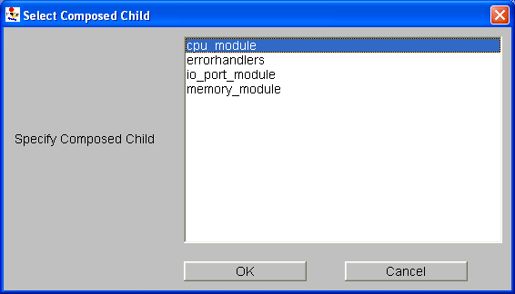
  6. 6.0 6.1 W. D. Obal II and W. H. Sanders. Measure-adaptive state-space construction methods. Performance Evaluation, 44:237–258, April 2001.
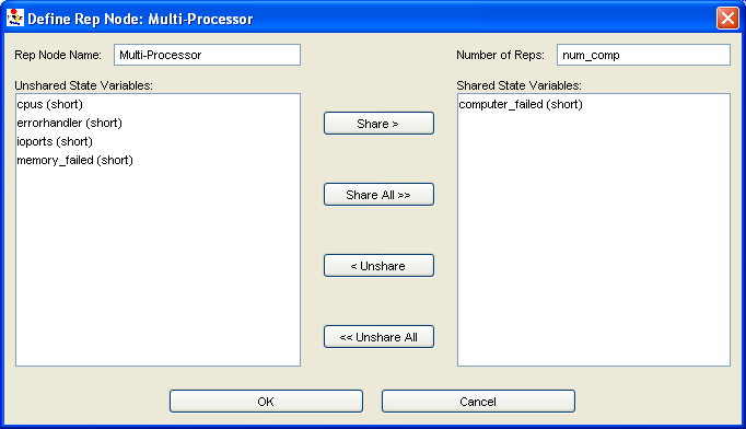
  7. W. J. Stewart. Introduction to the Numerical Solution of Markov Chains. Princeton University Press, 1994.
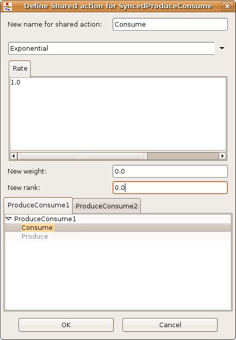
  8. A. Law and W. D. Kelton. Simulation modeling and Analysis. McGraw-Hill, 1991.