Examples
Contents
Fault-Tolerant Multiprocessor System
This section presents an example of a system that can be modeled using Möbius. It starts with a description of the system, and then guides you through one way to build a model of the system and solve it using both simulation and numerical solution. The example is intended to take you step-by-step through the process of creating and solving a model in Möbius, and to exhibit many of the capabilities and features of the tool.
System Description
The system under consideration is a highly redundant fault-tolerant multiprocessor system adapted from [1] and shown in <xr id="fig:ex_multiproc" />. At the highest level, the system consists of multiple computers. Each computer is composed of 3 memory modules, of which 1 is a spare module; 3 CPU units, of which 1 is a spare unit; 2 I/O ports, of which 1 is a spare port; and 2 non-redundant error-handling chips.
<figure id="fig:ex_multiproc">

Internally, each memory module consists of 41 RAM chips (2 of which are spare chips) and 2 interface chips. Each CPU unit and each I/O port consists of 6 non-redundant chips. The system is considered operational if at least 1 computer is operational. A computer is classified as operational if, of its components, at least 2 memory modules, at least 2 CPU units, at least 1 I/O port, and the 2 error-handling chips are functioning. A memory module is operational if at least 39 of its 41 RAM chips, and its 2 interface chips, are working.
Where there is redundancy (available spares) at any level of system hierarchy, there is a coverage factor associated with the component failure at that level. For example, following the parameter values used by Lee et al.[1], if one CPU unit fails, with probability 0.995 the failed unit will be replaced by the spare unit, if available, and the corresponding computer will continue to operate. On the other hand, there is also a 0.005 probability that the fault recovery mechanism will fail and the corresponding computer will cease to operate. <xr id="tab:ex_coverage" /> shows the redundant components and their associated fault coverage probability. Finally, the failure rate of every chip in the system, as in [1], is assumed to be 100 failures per billion hours1.
- 1 0.0008766 failures per year.
<figtable id="tab:ex_coverage">
| Redundant Component | Fault Coverage Probability |
|---|---|
| RAM Chip | 0.998 |
| Memory Module | 0.95 |
| CPU Unit | 0.995 |
| I/O Port | 0.99 |
| Computer | 0.95 |
Getting Started
A model of the system in this example is included with the Möbius distribution. Refer to Section C.1 for instructions on installing the example models. You are encouraged to open the model and follow the detailed discussions of its various components in the sections below.
From the Möbius Project Manager window, click Project Unarchive. A dialog will present a list of archived projects in the project directory. Choose Multiproc-Paper and hit Unarchive. After the project has been successfully unarchived, you will be prompted to resave the project using ProjectResave. At the dialog, choose Multiproc-Paper again, hit Resave, and wait until all components have been built. The Multiproc-Paper project editor will appear as shown in Figure 3.1.
Atomic Models
To build a model for an entire system, begin by defining SAN submodels to repre- sent the failures of various components in the system.
The SAN submodel of the CPUs is called cpu_module and is shown in <xr id="fig:ex_sancpu" />. To open this model, click the Atomic tab in the project panel, and then double-click on cpu_module or right-click on it and select Open. The places named cpus and computer_failed represent the current state of the CPUs and the current state of the multiprocessor system, respectively. That is, the number of tokens in cpus represents the number of operational CPUs in a given computer. Likewise, the number of tokens in computer_failed indicates the number of computers that have failed in the system. To open any of these places, right-click on the place and select Edit. This will bring up the Place Attributes dialog, in which you can edit the Name of the place and the initial marking (number of tokens) of the place. Note that the Tokens field can be specified with either a constant or a global variable name. For example, the place cpus has been initialized with three tokens, as each computer consists of three CPU units.
<figure id="fig:ex_sancpu">

To create a new place, either click the blue circle icon in the toolbar or select ElementsPlace from the menu. Then click where you would like the place to go in the editor. The Place Attributes dialog will appear, and you can edit the Name of the place as well as the initial marking of the place in the Tokens field, as described earlier. To delete a place, right-click on it and select Delete, and hit OK to confirm.
The places labeled ioports, errorhandlers, and memory_failed are also included in this model to aid in reducing the size of the state space for the overall system model by lumping as many failed states together as possible. Additional state lumping (beyond that provided by the reduced base model construction method) can be achieved because once a computer fails, there is no need to keep track of which component failure caused the computer failure. More specifically, because of the assumption that all internal components of the failed computer have failed, the states that represent a computer failure due to a failure of a CPU unit, a memory module, an I/O port, or an error-handling chip are combined into a single state. The marking of the combined state is reached by setting the number of tokens in each of the places cpus, ioports, and errorhandlers to zero, setting the number of tokens in memory_failed to 2, and incrementing the number of tokens in computer_failed.
The failure of a CPU unit corresponds to the completion of timed activity cpu_failure. To open this activity, right-click on it and select Edit. This will bring up the Timed Activity Attributes dialog. In this dialog, you can edit the name of the activity and the distribution of its firing delay in the Time distribution function field. For this activity, the Exponential distribution should be selected. The activity completion rate is shown in <xr id="tab:ex_cpuact" />. This rate corresponds to six2 times the failure rate of a chip times the number of operational CPU units in the computer. If a spare CPU unit is available (i.e., cpus->Mark() == 3), three cases are associated with the activity completion, as designated in the Case quantity field. To define the case probabilities, click on the appropriate case number’s tab and type the expression in the box. The expression for the case probability can be a constant, a global variable, or a C++ statement returning a value as in this example. The first case represents a successful coverage of a CPU unit failure. If that case occurs, the failed CPU unit is replaced by the spare unit, and its corresponding computer continues to operate. The second case represents the situation in which a CPU unit failure occurs that is not covered, but the failure of its corresponding computer is covered. If that happens and a spare computer is available, the failed computer is replaced by the spare computer and the system continues to operate. However, if no spare computer is available, the multiprocessor system fails. The third case represents the situation in which neither the CPU failure nor the corresponding computer failure is covered, resulting in a total system failure.
- 2 Remember that each CPU unit consists of 6 non-redundant chips.
<figtable id="tab:ex_cpuact">
| Activity | Distribution |
|---|---|
| cpu_failure | expon(0.0052596 * cpus->Mark()) |
On the other hand, if no spare CPU is available (i.e., cpus->Mark() == 2), then a CPU unit failure causes a computer failure. In this marking, two possible outcomes may result from the completion of activity cpu_failure. In the first, a spare computer is available, so that the computer failure can be covered. In the second, no spare computer is available, and system failure results. <xr id="tab:ex_cpucaseprob" /> shows the case numbers and the probabilities associated with each case for the activity cpu_failure. It is clear that the case probabilities are marking-dependent, since the coverage factors depend on the state of the system.
<figtable id="tab:ex_cpucaseprob">
| Case | Probability |
|---|---|
| cpu_failure | |
| 1 | if (cpus->Mark() == 3) return(0.995); else |
| 2 | if (cpus->Mark() == 3) return(0.00475); else |
| 3 | if (cpus->Mark() == 3) return(0.00025); else |
The input gate Input_Gate1 is used to determine whether the timed activity cpu_failure is enabled in the current marking, and hence can complete. The cpu_failure activity is enabled only if at least 2 working CPU units are available and their corresponding computer and the system have not failed. <xr id="tab:ex_cpuig1" /> shows the enabling predicate and function associated with this gate.
<figtable id="tab:ex_cpuig1">
| Gate | Enabling Predicate | Function |
|---|---|---|
| Input_Gate1 | (cpus->Mark()>1) && (memory_failed->Mark()<2) && |
identity |
The output gates OG1, OG2, and OG3 are used to determine the next marking based on the current marking and the case chosen when cpu_failure completes. They correspond to the different situations that arise because of the coverage or non-coverage of system components. <xr id="tab:ex_cpuog" /> lists the output gates and the function of each gate.
<figtable id="tab:ex_cpuog">
| Gate | Function |
|---|---|
| OG1 | if (cpus->Mark() == 3) cpus->Mark()--; |
| OG2 | cpus->Mark() = 0; ioports->Mark() = 0; errorhandlers->Mark() = 0; memory_failed->Mark() = 2; computer_failed->Mark()++; |
| OG3 | cpus->Mark() = 0; ioports->Mark() = 0; errorhandlers->Mark() = 0; memory_failed->Mark() = 2; computer_failed->Mark() = num_comp; |
In a SAN model, relationships between elements are designated by connecting lines or arcs. For example, places and input gates may be connected to an activity to indicate they are enabling conditions for the activity. An activity (or one of its cases) may be connected to a place or an output gate to indicate that upon completion of the activity, the marking of the place is affected or the output gate function is executed. It is not necessary to connect an output gate to a place whose marking the output gate function changes. Such a connection exists only to ease understanding of the model. To draw a connecting line or arc, choose either Straight Connection, Connected Line, or Spline Curve from the Elements menu. To connect two model elements using the first option, click on the first element and then click on the second element to draw a straight line between them. Using the second or third options, click on the first element, then click on one or more points between the two elements, and finally click on the second element. The Connected Line option will connect the two elements by linear interpolation of all user-defined points between them. The Spline Curve option is similar, but will connect the two elements with a smooth curve. The order in which the two elements are clicked is important, since the arcs, although drawn as undirected edges, are actually specified in a directed manner. For instance, to connect an input gate to an activity, the arc must be drawn from the input gate to the activity, and not vice versa. Also, there are some combinations of elements that cannot be connected, such as one place with another place or an input gate with an output gate.
Another way to model the failure of CPU modules would be to model the failure of a single CPU module as a SAN and replicate this model three times. However, since the failure of any chip inside the CPU module causes the CPU to fail, and each chip is assumed to have an exponentially distributed failure rate, the failure rate of one CPU module is just the sum of the failure rates of the 6 CPU chips. Therefore, modeling the failure of one CPU module, and then replicating this model three times, results in a model that is equivalent to the cpu_module submodel described above. Both approaches will generate the same number of states. In contrast, a significant state space reduction can be achieved by modeling one memory module as a SAN and replicating this model three times, instead of modeling the failure of the three memory modules in one SAN. The reason is that the failure of a single RAM chip does not cause the memory module to fail, so a memory module cannot be modeled as a single entity.
The SAN submodels of the I/O ports, the memory module, and the two error-handling chips are shown in <xr id="fig:ex_sanio" />, <xr id="fig:ex_sanmem" />, and <xr id="fig:ex_sanerror" />, respectively. The line of reasoning followed in modeling each of these components is similar to that followed in modeling the CPU modules. Note the similarity between the io_port_module and cpu_module SANs. A more detailed discussion of creating SAN models can be found in Section 4.1 of Building Models.
<figure id="fig:ex_sanio">

<figure id="fig:ex_sanmem">

<figure id="fig:ex_sanerror">

Composed Model
Now the replicate and join operations previously defined (see Section 5.1 of Building Models) are used to construct a complete composed model from the atomic models. <xr id="fig:ex_composed" /> shows the multi_proc composed model for the multiprocessor system. To open this model click the Composed tab in the project panel, and double-click on multi_proc or right-click on it and select Open.
<figure id="fig:ex_composed">

The leaf nodes represent the individual submodels, or atomic models, that were defined in the previous section. The memory_module is replicated 3 times, corresponding to the number of memory modules in each computer, with the places computer_failed and memory_failed (see <xr id="fig:ex_sanmem" />) held in common among all the replicas. You can see where that is set by right-clicking on the Rep node whose child is the memory_module submodel, and choosing Edit. The Define Rep Node: REP1 window will appear. Here the name of the Rep node is specified as Rep1, and the Number of Reps is specified as the global variable num_mem_mod, which is later defined to be 3 in Section 1.6. The two lists Unshared State Variables and Shared State Variables define which state variables are shared, or held in common, among all replicas. To move a state variable from one list to the other use either the Share > or < Unshare button. To move all state variables use the Share All >> or << Unshare All button. You can create a new Rep node by selecting the red ![]() icon from the toolbar or choosing ElementsRep from the menu. Then click inside the editor where the Rep node is to be placed and specify the name of the node and the number of Reps in the Define Rep Node dialog. A Rep node must have as its child either an atomic model or another composed model. Click on the black
icon from the toolbar or choosing ElementsRep from the menu. Then click inside the editor where the Rep node is to be placed and specify the name of the node and the number of Reps in the Define Rep Node dialog. A Rep node must have as its child either an atomic model or another composed model. Click on the black ![]() icon in the toolbar or select ElementsSubmodel to add a submodel. Then you can draw a connecting line from the Rep node to the child submodel in the same way that you would draw connecting lines in the atomic model editor (see Section 1.3). Once a Rep node is given a child, the shared state variables can be defined by editing the Rep node again.
icon in the toolbar or select ElementsSubmodel to add a submodel. Then you can draw a connecting line from the Rep node to the child submodel in the same way that you would draw connecting lines in the atomic model editor (see Section 1.3). Once a Rep node is given a child, the shared state variables can be defined by editing the Rep node again.
The three memory modules are then joined to the I/O ports model (<xr id="fig:ex_sanio" />), CPUs failure model (<xr id="fig:ex_sancpu" />), and error-handler model (<xr id="fig:ex_sanerror" />) to form a model of a computer. In the Join node, places with a common name are shared, and thus treated as single places among all system submodels. To open this node, right-click on the blue Join node and select Edit. This will bring up the Define Join Node dialog. Here, the Join node name is specified as Join1 and shared state variables can be created. The Join State Variables list shows all state variables that are shared across multiple submodels in the Join. Clicking on a shared variable in this list will display the corresponding name of the shared variable in each of the submodels among which it is shared under the Submodel Variables list. The # Shared column indicates how many submodels share each Join state variable. To share a state variable among submodels in a Join, click the Create New Shared Variable button, give a name for the new variable, and select the submodel state variables that are to be shared. In this example, places with a common name across different submodels are shared; this is achieved with the Share All Similar Variables button. A new Join node can be created by clicking on the blue ![]() icon in the toolbar or selecting Join from the Elements menu. Then the Join node must be connected to its children nodes with arcs as discussed previously. A Join node can have as its children submodels, Rep nodes, or other Join nodes.
icon in the toolbar or selecting Join from the Elements menu. Then the Join node must be connected to its children nodes with arcs as discussed previously. A Join node can have as its children submodels, Rep nodes, or other Join nodes.
Finally, the joined SAN model of one computer is replicated num_comp times by the ‘Rep2’ node to generate the complete model of the multiprocessor system. More information about creating composed models and the composed model editor can be found in Section 5 of Building Models.
Reward Variables
After the composed model of the multiprocessor system has been built, the next step in the model construction process is to define reward variables. Reward variables permit us to compute interesting measures from the model. This example, for instance, focuses on measuring the reliability of the multiprocessor system over a 20-year mission time. The system is considered unreliable by time t if all of the num_comp computers in the system have failed. In terms of this model, the system is unreliable when there are num_comp tokens in place computer_failed.
To define the reliability variable, click on Reward in the project panel, then click New (either in the toolbar or by right-clicking on Reward and selecting New) and specify the new performance variable model name. Or, to view the existing performance variable model for this example, click the Reward tab in the Project panel. All previously defined variables are listed under this tab. The reliability variable should already have been defined, and you can open it for revision either by double-clicking on the variable MultiProc_PV or by choosing it and then clicking on the Open button on the panel. That will open up the Reward Editor for the variable.
On the left-hand side of the Reward Editor window, there is a Variable List sub-window containing all defined reward variables for this model. In the example, unreliability is the only variable. Choose it for revision by clicking on it once. Then click on the Submodels tab to choose the submodels on which the reward is to be computed. Because unreliability is defined on the place computer_failed in the submodel cpu_module, choose this submodel by clicking on it once (see <xr id="fig:ExampleSubmodelTab" />).
<figure id="fig:ExampleSubmodelTab">

Next, to define the rate reward for unreliability, click on the tab Rate Rewards. This will bring up two sub-windows. The top sub-window lists all available state variables in the model on which rate rewards can be defined. The bottom sub-window, Reward Function, is a text area for entering C++ code for computing reward for the currently selected reward variable (see <xr id="fig:ExampleRateTab" />). In this example, a reward of (1/num_comp) should be returned when all of the computers have failed, because the reward is evaluated over all submodels in the composed model. That is, a reward of (1/num_comp) is accumulated once for each computer, or a total of num_comp times, for a total reward of 1. Thus, the reward for a state in which all computers have failed is 1, and the mean unreliability of the system (for example) can be found by calculating the mean of this reward variable. The C++ code that should be entered in this sub-window is
if (cpu_module->computer_failed->Mark() == num_comp)
{
- return 1.0/num_comp;
}
<figure id="fig:ExampleRateTab">

Now click the Simulation tab to view the parameters for simulation. Since the goal is to measure the unreliability of the system at a particular time (20 years), the Type has been set to Instant of Time and the Start time to 20.0 as in <xr id="fig:ex_rewardsim" />. You can ignore the Estimation and Confidence tabs for now.
<figure id="fig:ex_rewardsim">

Möbius
Möbius
Motivation
Solution
Graph
Edit Möbius Documentation
“” –
<equation id="eqn:binom" shownumber>
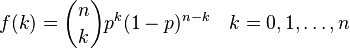
</equation>
Sort of like <xr id="eqn:binom" />, but not really.
References
- ↑ 1.0 1.1 1.2 D. Lee, J. Abraham, D. Rennels, and G. Gilley. A numerical technique for the evaluation of large, closed fault-tolerant systems. In Dependable Computing for Critical Applications, pages 95–114. Springer-Verlag, Wien, 1992.
Contents
Fault-Tolerant Multiprocessor System[edit]
This section presents an example of a system that can be modeled using Möbius. It starts with a description of the system, and then guides you through one way to build a model of the system and solve it using both simulation and numerical solution. The example is intended to take you step-by-step through the process of creating and solving a model in Möbius, and to exhibit many of the capabilities and features of the tool.
System Description[edit]
The system under consideration is a highly redundant fault-tolerant multiprocessor system adapted from [1] and shown in <xr id="fig:ex_multiproc" />. At the highest level, the system consists of multiple computers. Each computer is composed of 3 memory modules, of which 1 is a spare module; 3 CPU units, of which 1 is a spare unit; 2 I/O ports, of which 1 is a spare port; and 2 non-redundant error-handling chips.
<figure id="fig:ex_multiproc">
Internally, each memory module consists of 41 RAM chips (2 of which are spare chips) and 2 interface chips. Each CPU unit and each I/O port consists of 6 non-redundant chips. The system is considered operational if at least 1 computer is operational. A computer is classified as operational if, of its components, at least 2 memory modules, at least 2 CPU units, at least 1 I/O port, and the 2 error-handling chips are functioning. A memory module is operational if at least 39 of its 41 RAM chips, and its 2 interface chips, are working.
Where there is redundancy (available spares) at any level of system hierarchy, there is a coverage factor associated with the component failure at that level. For example, following the parameter values used by Lee et al.[1], if one CPU unit fails, with probability 0.995 the failed unit will be replaced by the spare unit, if available, and the corresponding computer will continue to operate. On the other hand, there is also a 0.005 probability that the fault recovery mechanism will fail and the corresponding computer will cease to operate. <xr id="tab:ex_coverage" /> shows the redundant components and their associated fault coverage probability. Finally, the failure rate of every chip in the system, as in [1], is assumed to be 100 failures per billion hours1.
- 1 0.0008766 failures per year.
<figtable id="tab:ex_coverage">
| Redundant Component | Fault Coverage Probability |
|---|---|
| RAM Chip | 0.998 |
| Memory Module | 0.95 |
| CPU Unit | 0.995 |
| I/O Port | 0.99 |
| Computer | 0.95 |
Getting Started[edit]
A model of the system in this example is included with the Möbius distribution. Refer to Section C.1 for instructions on installing the example models. You are encouraged to open the model and follow the detailed discussions of its various components in the sections below.
From the Möbius Project Manager window, click ProjectUnarchive. A dialog will present a list of archived projects in the project directory. Choose Multiproc-Paper and hit Unarchive. After the project has been successfully unarchived, you will be prompted to resave the project using ProjectResave. At the dialog, choose Multiproc-Paper again, hit Resave, and wait until all components have been built. The Multiproc-Paper project editor will appear as shown in Figure 3.1.
Atomic Models[edit]
To build a model for an entire system, begin by defining SAN submodels to repre- sent the failures of various components in the system.
The SAN submodel of the CPUs is called cpu_module and is shown in <xr id="fig:ex_sancpu" />. To open this model, click the Atomic tab in the project panel, and then double-click on cpu_module or right-click on it and select Open. The places named cpus and computer_failed represent the current state of the CPUs and the current state of the multiprocessor system, respectively. That is, the number of tokens in cpus represents the number of operational CPUs in a given computer. Likewise, the number of tokens in computer_failed indicates the number of computers that have failed in the system. To open any of these places, right-click on the place and select Edit. This will bring up the Place Attributes dialog, in which you can edit the Name of the place and the initial marking (number of tokens) of the place. Note that the Tokens field can be specified with either a constant or a global variable name. For example, the place cpus has been initialized with three tokens, as each computer consists of three CPU units.
<figure id="fig:ex_sancpu">
To create a new place, either click the blue circle icon in the toolbar or select ElementsPlace from the menu. Then click where you would like the place to go in the editor. The Place Attributes dialog will appear, and you can edit the Name of the place as well as the initial marking of the place in the Tokens field, as described earlier. To delete a place, right-click on it and select Delete, and hit OK to confirm.
The places labeled ioports, errorhandlers, and memory_failed are also included in this model to aid in reducing the size of the state space for the overall system model by lumping as many failed states together as possible. Additional state lumping (beyond that provided by the reduced base model construction method) can be achieved because once a computer fails, there is no need to keep track of which component failure caused the computer failure. More specifically, because of the assumption that all internal components of the failed computer have failed, the states that represent a computer failure due to a failure of a CPU unit, a memory module, an I/O port, or an error-handling chip are combined into a single state. The marking of the combined state is reached by setting the number of tokens in each of the places cpus, ioports, and errorhandlers to zero, setting the number of tokens in memory_failed to 2, and incrementing the number of tokens in computer_failed.
The failure of a CPU unit corresponds to the completion of timed activity cpu_failure. To open this activity, right-click on it and select Edit. This will bring up the Timed Activity Attributes dialog. In this dialog, you can edit the name of the activity and the distribution of its firing delay in the Time distribution function field. For this activity, the Exponential distribution should be selected. The activity completion rate is shown in <xr id="tab:ex_cpuact" />. This rate corresponds to six2 times the failure rate of a chip times the number of operational CPU units in the computer. If a spare CPU unit is available (i.e., cpus->Mark() == 3), three cases are associated with the activity completion, as designated in the Case quantity field. To define the case probabilities, click on the appropriate case number’s tab and type the expression in the box. The expression for the case probability can be a constant, a global variable, or a C++ statement returning a value as in this example. The first case represents a successful coverage of a CPU unit failure. If that case occurs, the failed CPU unit is replaced by the spare unit, and its corresponding computer continues to operate. The second case represents the situation in which a CPU unit failure occurs that is not covered, but the failure of its corresponding computer is covered. If that happens and a spare computer is available, the failed computer is replaced by the spare computer and the system continues to operate. However, if no spare computer is available, the multiprocessor system fails. The third case represents the situation in which neither the CPU failure nor the corresponding computer failure is covered, resulting in a total system failure.
- 2 Remember that each CPU unit consists of 6 non-redundant chips.
<figtable id="tab:ex_cpuact">
| Activity | Distribution |
|---|---|
| cpu_failure | expon(0.0052596 * cpus->Mark()) |
On the other hand, if no spare CPU is available (i.e., cpus->Mark() == 2), then a CPU unit failure causes a computer failure. In this marking, two possible outcomes may result from the completion of activity cpu_failure. In the first, a spare computer is available, so that the computer failure can be covered. In the second, no spare computer is available, and system failure results. <xr id="tab:ex_cpucaseprob" /> shows the case numbers and the probabilities associated with each case for the activity cpu_failure. It is clear that the case probabilities are marking-dependent, since the coverage factors depend on the state of the system.
<figtable id="tab:ex_cpucaseprob">
| Case | Probability |
|---|---|
| cpu_failure | |
| 1 | if (cpus->Mark() == 3) return(0.995); else |
| 2 | if (cpus->Mark() == 3) return(0.00475); else |
| 3 | if (cpus->Mark() == 3) return(0.00025); else |
The input gate Input_Gate1 is used to determine whether the timed activity cpu_failure is enabled in the current marking, and hence can complete. The cpu_failure activity is enabled only if at least 2 working CPU units are available and their corresponding computer and the system have not failed. <xr id="tab:ex_cpuig1" /> shows the enabling predicate and function associated with this gate.
<figtable id="tab:ex_cpuig1">
| Gate | Enabling Predicate | Function |
|---|---|---|
| Input_Gate1 | (cpus->Mark()>1) && (memory_failed->Mark()<2) && |
identity |
The output gates OG1, OG2, and OG3 are used to determine the next marking based on the current marking and the case chosen when cpu_failure completes. They correspond to the different situations that arise because of the coverage or non-coverage of system components. <xr id="tab:ex_cpuog" /> lists the output gates and the function of each gate.
<figtable id="tab:ex_cpuog">
| Gate | Function |
|---|---|
| OG1 | if (cpus->Mark() == 3) cpus->Mark()--; |
| OG2 | cpus->Mark() = 0; ioports->Mark() = 0; errorhandlers->Mark() = 0; memory_failed->Mark() = 2; computer_failed->Mark()++; |
| OG3 | cpus->Mark() = 0; ioports->Mark() = 0; errorhandlers->Mark() = 0; memory_failed->Mark() = 2; computer_failed->Mark() = num_comp; |
In a SAN model, relationships between elements are designated by connecting lines or arcs. For example, places and input gates may be connected to an activity to indicate they are enabling conditions for the activity. An activity (or one of its cases) may be connected to a place or an output gate to indicate that upon completion of the activity, the marking of the place is affected or the output gate function is executed. It is not necessary to connect an output gate to a place whose marking the output gate function changes. Such a connection exists only to ease understanding of the model. To draw a connecting line or arc, choose either Straight Connection, Connected Line, or Spline Curve from the Elements menu. To connect two model elements using the first option, click on the first element and then click on the second element to draw a straight line between them. Using the second or third options, click on the first element, then click on one or more points between the two elements, and finally click on the second element. The Connected Line option will connect the two elements by linear interpolation of all user-defined points between them. The Spline Curve option is similar, but will connect the two elements with a smooth curve. The order in which the two elements are clicked is important, since the arcs, although drawn as undirected edges, are actually specified in a directed manner. For instance, to connect an input gate to an activity, the arc must be drawn from the input gate to the activity, and not vice versa. Also, there are some combinations of elements that cannot be connected, such as one place with another place or an input gate with an output gate.
Another way to model the failure of CPU modules would be to model the failure of a single CPU module as a SAN and replicate this model three times. However, since the failure of any chip inside the CPU module causes the CPU to fail, and each chip is assumed to have an exponentially distributed failure rate, the failure rate of one CPU module is just the sum of the failure rates of the 6 CPU chips. Therefore, modeling the failure of one CPU module, and then replicating this model three times, results in a model that is equivalent to the cpu_module submodel described above. Both approaches will generate the same number of states. In contrast, a significant state space reduction can be achieved by modeling one memory module as a SAN and replicating this model three times, instead of modeling the failure of the three memory modules in one SAN. The reason is that the failure of a single RAM chip does not cause the memory module to fail, so a memory module cannot be modeled as a single entity.
The SAN submodels of the I/O ports, the memory module, and the two error-handling chips are shown in <xr id="fig:ex_sanio" />, <xr id="fig:ex_sanmem" />, and <xr id="fig:ex_sanerror" />, respectively. The line of reasoning followed in modeling each of these components is similar to that followed in modeling the CPU modules. Note the similarity between the io_port_module and cpu_module SANs. A more detailed discussion of creating SAN models can be found in Section 4.1 of Building Models.
<figure id="fig:ex_sanio">
<figure id="fig:ex_sanmem">
<figure id="fig:ex_sanerror">
Composed Model[edit]
Now the replicate and join operations previously defined (see Section 5.1 of Building Models) are used to construct a complete composed model from the atomic models. <xr id="fig:ex_composed" /> shows the multi_proc composed model for the multiprocessor system. To open this model click the Composed tab in the project panel, and double-click on multi_proc or right-click on it and select Open.
<figure id="fig:ex_composed">
The leaf nodes represent the individual submodels, or atomic models, that were defined in the previous section. The memory_module is replicated 3 times, corresponding to the number of memory modules in each computer, with the places computer_failed and memory_failed (see <xr id="fig:ex_sanmem" />) held in common among all the replicas. You can see where that is set by right-clicking on the Rep node whose child is the memory_module submodel, and choosing Edit. The Define Rep Node: REP1 window will appear. Here the name of the Rep node is specified as Rep1, and the Number of Reps is specified as the global variable num_mem_mod, which is later defined to be 3 in Section 1.6. The two lists Unshared State Variables and Shared State Variables define which state variables are shared, or held in common, among all replicas. To move a state variable from one list to the other use either the Share > or < Unshare button. To move all state variables use the Share All >> or << Unshare All button. You can create a new Rep node by selecting the red ![]() icon from the toolbar or choosing ElementsRep from the menu. Then click inside the editor where the Rep node is to be placed and specify the name of the node and the number of Reps in the Define Rep Node dialog. A Rep node must have as its child either an atomic model or another composed model. Click on the black
icon from the toolbar or choosing ElementsRep from the menu. Then click inside the editor where the Rep node is to be placed and specify the name of the node and the number of Reps in the Define Rep Node dialog. A Rep node must have as its child either an atomic model or another composed model. Click on the black ![]() icon in the toolbar or select ElementsSubmodel to add a submodel. Then you can draw a connecting line from the Rep node to the child submodel in the same way that you would draw connecting lines in the atomic model editor (see Section 1.3). Once a Rep node is given a child, the shared state variables can be defined by editing the Rep node again.
icon in the toolbar or select ElementsSubmodel to add a submodel. Then you can draw a connecting line from the Rep node to the child submodel in the same way that you would draw connecting lines in the atomic model editor (see Section 1.3). Once a Rep node is given a child, the shared state variables can be defined by editing the Rep node again.
The three memory modules are then joined to the I/O ports model (<xr id="fig:ex_sanio" />), CPUs failure model (<xr id="fig:ex_sancpu" />), and error-handler model (<xr id="fig:ex_sanerror" />) to form a model of a computer. In the Join node, places with a common name are shared, and thus treated as single places among all system submodels. To open this node, right-click on the blue Join node and select Edit. This will bring up the Define Join Node dialog. Here, the Join node name is specified as Join1 and shared state variables can be created. The Join State Variables list shows all state variables that are shared across multiple submodels in the Join. Clicking on a shared variable in this list will display the corresponding name of the shared variable in each of the submodels among which it is shared under the Submodel Variables list. The # Shared column indicates how many submodels share each Join state variable. To share a state variable among submodels in a Join, click the Create New Shared Variable button, give a name for the new variable, and select the submodel state variables that are to be shared. In this example, places with a common name across different submodels are shared; this is achieved with the Share All Similar Variables button. A new Join node can be created by clicking on the blue ![]() icon in the toolbar or selecting Join from the Elements menu. Then the Join node must be connected to its children nodes with arcs as discussed previously. A Join node can have as its children submodels, Rep nodes, or other Join nodes.
icon in the toolbar or selecting Join from the Elements menu. Then the Join node must be connected to its children nodes with arcs as discussed previously. A Join node can have as its children submodels, Rep nodes, or other Join nodes.
Finally, the joined SAN model of one computer is replicated num_comp times by the ‘Rep2’ node to generate the complete model of the multiprocessor system. More information about creating composed models and the composed model editor can be found in Section 5 of Building Models.
Reward Variables[edit]
After the composed model of the multiprocessor system has been built, the next step in the model construction process is to define reward variables. Reward variables permit us to compute interesting measures from the model. This example, for instance, focuses on measuring the reliability of the multiprocessor system over a 20-year mission time. The system is considered unreliable by time t if all of the num_comp computers in the system have failed. In terms of this model, the system is unreliable when there are num_comp tokens in place computer_failed.
To define the reliability variable, click on Reward in the project panel, then click New (either in the toolbar or by right-clicking on Reward and selecting New) and specify the new performance variable model name. Or, to view the existing performance variable model for this example, click the Reward tab in the Project panel. All previously defined variables are listed under this tab. The reliability variable should already have been defined, and you can open it for revision either by double-clicking on the variable MultiProc_PV or by choosing it and then clicking on the Open button on the panel. That will open up the Reward Editor for the variable.
On the left-hand side of the Reward Editor window, there is a Variable List sub-window containing all defined reward variables for this model. In the example, unreliability is the only variable. Choose it for revision by clicking on it once. Then click on the Submodels tab to choose the submodels on which the reward is to be computed. Because unreliability is defined on the place computer_failed in the submodel cpu_module, choose this submodel by clicking on it once (see <xr id="fig:ExampleSubmodelTab" />).
<figure id="fig:ExampleSubmodelTab">
Next, to define the rate reward for unreliability, click on the tab Rate Rewards. This will bring up two sub-windows. The top sub-window lists all available state variables in the model on which rate rewards can be defined. The bottom sub-window, Reward Function, is a text area for entering C++ code for computing reward for the currently selected reward variable (see <xr id="fig:ExampleRateTab" />). In this example, a reward of (1/num_comp) should be returned when all of the computers have failed, because the reward is evaluated over all submodels in the composed model. That is, a reward of (1/num_comp) is accumulated once for each computer, or a total of num_comp times, for a total reward of 1. Thus, the reward for a state in which all computers have failed is 1, and the mean unreliability of the system (for example) can be found by calculating the mean of this reward variable. The C++ code that should be entered in this sub-window is
if (cpu_module->computer_failed->Mark() == num_comp)
{
- return 1.0/num_comp;
}
<figure id="fig:ExampleRateTab">
Now click the Simulation tab to view the parameters for simulation. Since the goal is to measure the unreliability of the system at a particular time (20 years), the Type has been set to Instant of Time and the Start time to 20.0 as in <xr id="fig:ex_rewardsim" />. You can ignore the Estimation and Confidence tabs for now.
<figure id="fig:ex_rewardsim">
Möbius
Möbius[edit]
Motivation[edit]
Solution[edit]
Graph
Edit Möbius Documentation
“” –
<equation id="eqn:binom" shownumber>
</equation>
Sort of like <xr id="eqn:binom" />, but not really.