Solving Models
Contents
How to pick the solver
Möbius provides two types of solvers for obtaining solutions on measures of interest: simulation and numerical solvers. The choice of which type of solvers to use depends on a number of factors. More details on these factors are provided in the sections on simulation (Section 3) and numerical solvers (Section 4).
In general, the simulation solver can be used to solve all models that were built in Möbius, whereas numerical solvers can be used on only those modes that have only exponentially and deterministically distributed actions. In addition, simulation may be used on models that have arbitrarily large state-space descriptions, whereas numerical solvers are limited to models that have finite, small state-space description (that may be held in core memory). Furthermore, simulation may be more useful than numerical solvers for stiff models.
On the other hand, all numerical solvers in Möbius are capable of providing exact solutions (up to machine precision), whereas simulation provides statistically accurate solutions within some user-specifiable confidence interval. The desired accuracy of the computed solutions can be increased without excessive increase in computation time for most numerical solvers, while an increase in accuracy may be quite expensive for simulation. Additionally, full distributions may be computed for results from the numerical solvers, but usually not for results from simulation. Furthermore, for models in which numerical solvers are applicable, detection of rare events incurs no extra costs and requires no special techniques, whereas such computation by simulation is extremely expensive and uses the statistical technique of importance sampling.
Transformers
Introduction
Some of the solution techniques within Möbius, such as the simulator, operate directly on the model representation defined using the Atomic and Composed editors described in earlier chapters of the manual. These solvers operator on the model using the Möbius model-level abstract functional interface. There are other solution techniques, specifically the numerical solvers described in the next chapter, which require a different representation of the model as an input. Instead of operating on the high-level model description, numerical solution techniques use a lower-level, state space representation, namely the Markov chain.
Flat State Space Generator
The flat state space generator1 is used to generate the state space of the discrete-state stochastic process inherent in a model. The state space consists of the set of all states and the transitions between them. Once the state space has been generated, an appropriate analytical solver can be chosen to solve the model, as explained in Section 4.
- 1 This was the only state space generator (SSG) available prior to version 1.6.0 and it was simply called the state space generator. From that version on, it is called the flat state space generator.
While simulation can be applied to models with any underlying stochastic process, numerical solution requires that the model satisfy one of the following properties:
- All timed actions are exponentially distributed (Markov processes).
- All timed actions are deterministic or exponentially distributed, with at most one deterministic action enabled at any time. Furthermore, the firing delay of the deterministic actions may not be state-dependent.
The only restrictions on the use of instantaneous (zero-timed) actions are that the model must begin in a stable state, and the model must be stabilizing and well-specified [1]. It should also be noted that the reactivation predicates (see Section 4.1.1 of Building Models) must preserve the Markov property. In other words, the timed actions in the model must be reactivated so that the firing time distributions depend only on the current state, and not on any past state. That rule pertains only to timed actions with firing delays that are state-dependent.
The flat state space generator consists of a window with two tabs, SSG Info and SSG Output, which are discussed below.
Parameters
The SSG Info tab (<xr id="fig:ssg_info" />) is presented when you open the interface, and allows you to specify options and edit input to the state space generator.
<figure id="fig:ssg_info">

- The Study Name text box specifies the name of the child study. This box will show the name of the study you selected to be the child when you created the new solver. You can change the child study by typing a new name in the box or clicking the Browse button and selecting the solver child from the list of available studies.
- The Experiment List box displays the list of active experiments in the study, and will be updated upon any changes made through the Experiment Activator button.
- The Experiment Activator button can be used to activate or deactivate experiments defined in the child study, and provides the same functionality as the study editor Experiment Activator described in Section 7.3 of Building Models.
- The Run Name text box specifies the name for a particular run of the state space generator. This field is used to name trace files and output files (see below), and defaults to “Results” when a new solver is created. If no run name is given, the solver name will be used.
- The Build Type pull-down menu is used to choose whether the generator should be run in Optimize or Normal mode. In normal mode, the model is compiled without compiler optimizations, and you can specify various levels of output by changing the trace level, as explained below. This mode is useful for testing or debugging a model, as a text file named
 Run Name
 _Expx_trace.txt will be created for each experiment and contain a trace of the generation. In optimize mode, the model is compiled with maximum compiler optimizations, and all trace output is disabled for maximum performance. Running the generator will write over any data from a previous run of the same name, so change the Run Name field if you wish to save output/traces from an earlier run.
- The Build Type pull-down menu is used to choose whether the generator should be run in Optimize or Normal mode. In normal mode, the model is compiled without compiler optimizations, and you can specify various levels of output by changing the trace level, as explained below. This mode is useful for testing or debugging a model, as a text file named
- The Trace Level pull-down menu is enabled only when Normal mode is selected as the Build Type. This feature is useful for debugging purposes, as it allows you to select the amount of detail the generator will produce in the trace. The five options for Trace Level are:
- Level 0: None No detail in the trace. This would produce the same output as if optimize mode were selected.
- Level 1: Action Name For each new state discovered, prints the names of the actions enabled in this state. These are the actions that are fired when all possible next states from the current state are being explored.
- Level 2: Level 1 + State The same as Level 1, with the addition that the current state is printed along with the actions that are enabled in the state.
- Level 3 has not yet been implemented in Möbius.
- Level 4: All The same as Level 2, with the addition that the next states reachable from each state currently being explored are also printed.
- While a higher trace level will produce more detail in the generator trace and aid in debugging a model, it comes at the cost of slower execution time and larger file size.
- The Hash Value text box is used by the hash table data structure, which stores the set of discovered states in the generation algorithm. This number specifies the point at which the hash table is resized. Specifically, it is the ratio of the number of states discovered to the size of the hash table when a resizing2 occurs. The default value of
 , which means that the hash table is resized when it becomes half full, should suffice for most purposes.
- The Hash Value text box is used by the hash table data structure, which stores the set of discovered states in the generation algorithm. This number specifies the point at which the hash table is resized. Specifically, it is the ratio of the number of states discovered to the size of the hash table when a resizing2 occurs. The default value of
- 2 A resizing rehashes and roughly doubles the size of the hash table.
- The Flag Absorbing States checkbox, when selected, will print an alert when an absorbing state is encountered. An absorbing state is one for which there are no next (successor) states.
- The Place Comments in Output checkbox, when selected, will put the user-entered comments in the generator output/trace. If the box is not checked, no comments will appear, regardless of whether any have been entered.
- The Edit Comments button allows you to enter your own comments for a run of the generator. Clicking this button brings up the window shown in <xr id="fig:ssg_commentbox" />. Type any helpful comments in the box and hit OK to save or Cancel to discard the comments. The Clear button will clear all the text from the comment box.
<figure id="fig:ssg_commentbox">

- The Place Comments in Output checkbox, when selected, will put the user-entered comments in the generator output/trace. If the box is not checked, no comments will appear, regardless of whether any have been entered.
- The Experiment List box displays the list of active experiments in the study, and will be updated upon any changes made through the Experiment Activator button.
Generation
Clicking the Start State Space Generation button switches the view to the SSG Output tab and begins the process of generating the state space. The output window appears in <xr id="fig:ssg_output" />.
<figure id="fig:ssg_output">

First the models3 are compiled and the generator is built. For each active experiment, the values of the global variables are printed; if normal mode is being used, information about the trace level and hash table is also displayed. Then the state space is generated for the experiment. While it is being generated, the States Generated box and progress bar at the bottom of the dialog indicate the number of states that have been discovered. This number is updated once for every 1,000 states generated and when generation is complete. At any time, you may use the Stop button to terminate the run. A text file named Run Name_output.txt will be created. It will mirror the data output in the GUI.
- 3 Here models refers to the atomic/composed models, performance variable, and study.
A final remark is in order about the notion of state during generation of the state space of the stochastic process. In Möbius, a state is defined as the values of the state variables along with the impulse reward (see Section 6.1.1 of Building Models) associated with the action whose firing led to that state. Therefore, for a model on which impulse rewards have been defined, if two different actions may fire in a given state and lead to the same next state, they give rise to two unique states in the state space. The reason is that when impulse rewards are defined, the state space generator must store information about the last action fired. The result is a larger state space for models on which impulse rewards have been defined. It is important to realize this when analyzing the size of the generated state space.
Command line options
The flat state space generator is usually run from the GUI. However, since the models are compiled and linked with the generator libraries to form an executable, the generator can also be run from the command line (e.g., from a system shell/terminal window). The executable is found in the directory
- Möbius Project Root/Project Name/Solver/Solver Name/
-
and is named Solver NameGen_Arch[_debug], where Arch is the system architecture (Windows, Linux, or Solaris) and _debug is appended if you build the flat state space generator in normal mode. The command line options and their arguments are as follows:
-P experimentfilepath
- Place the created experiment files in the directory specified by experimentfilepath. This argument can be a relative path. By default, the experiment files will be placed in the current directory, but you can specify a path using the option “-E.”
-N experimentname
- Use experimentname to name the experiment files created. These files will have extensions .arm or .var, and will be placed in the directory specified by the “-E” option.
-B experimentnumber
Graph
Graph
Graph
Graph
Graph
Graph
Möbius
Möbius
Motivation
Solution
Graph
Edit Möbius Documentation
“” –
<equation id="eqn:binom" shownumber>
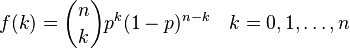
</equation>
Sort of like <xr id="eqn:binom" />, but not really.
References
- ↑ W. H. Sanders. Construction and Solution of Performability Models Based on Stochastic Activity Networks. PhD thesis, University of Michigan, Ann Arbor, Michigan, 1988.
Contents
How to pick the solver[edit]
Möbius provides two types of solvers for obtaining solutions on measures of interest: simulation and numerical solvers. The choice of which type of solvers to use depends on a number of factors. More details on these factors are provided in the sections on simulation (Section 3) and numerical solvers (Section 4).
In general, the simulation solver can be used to solve all models that were built in Möbius, whereas numerical solvers can be used on only those modes that have only exponentially and deterministically distributed actions. In addition, simulation may be used on models that have arbitrarily large state-space descriptions, whereas numerical solvers are limited to models that have finite, small state-space description (that may be held in core memory). Furthermore, simulation may be more useful than numerical solvers for stiff models.
On the other hand, all numerical solvers in Möbius are capable of providing exact solutions (up to machine precision), whereas simulation provides statistically accurate solutions within some user-specifiable confidence interval. The desired accuracy of the computed solutions can be increased without excessive increase in computation time for most numerical solvers, while an increase in accuracy may be quite expensive for simulation. Additionally, full distributions may be computed for results from the numerical solvers, but usually not for results from simulation. Furthermore, for models in which numerical solvers are applicable, detection of rare events incurs no extra costs and requires no special techniques, whereas such computation by simulation is extremely expensive and uses the statistical technique of importance sampling.
Transformers[edit]
Introduction[edit]
Some of the solution techniques within Möbius, such as the simulator, operate directly on the model representation defined using the Atomic and Composed editors described in earlier chapters of the manual. These solvers operator on the model using the Möbius model-level abstract functional interface. There are other solution techniques, specifically the numerical solvers described in the next chapter, which require a different representation of the model as an input. Instead of operating on the high-level model description, numerical solution techniques use a lower-level, state space representation, namely the Markov chain.
Flat State Space Generator[edit]
The flat state space generator1 is used to generate the state space of the discrete-state stochastic process inherent in a model. The state space consists of the set of all states and the transitions between them. Once the state space has been generated, an appropriate analytical solver can be chosen to solve the model, as explained in Section 4.
- 1 This was the only state space generator (SSG) available prior to version 1.6.0 and it was simply called the state space generator. From that version on, it is called the flat state space generator.
While simulation can be applied to models with any underlying stochastic process, numerical solution requires that the model satisfy one of the following properties:
- All timed actions are exponentially distributed (Markov processes).
- All timed actions are deterministic or exponentially distributed, with at most one deterministic action enabled at any time. Furthermore, the firing delay of the deterministic actions may not be state-dependent.
The only restrictions on the use of instantaneous (zero-timed) actions are that the model must begin in a stable state, and the model must be stabilizing and well-specified [1]. It should also be noted that the reactivation predicates (see Section 4.1.1 of Building Models) must preserve the Markov property. In other words, the timed actions in the model must be reactivated so that the firing time distributions depend only on the current state, and not on any past state. That rule pertains only to timed actions with firing delays that are state-dependent.
The flat state space generator consists of a window with two tabs, SSG Info and SSG Output, which are discussed below.
Parameters[edit]
The SSG Info tab (<xr id="fig:ssg_info" />) is presented when you open the interface, and allows you to specify options and edit input to the state space generator.
<figure id="fig:ssg_info">
- The Study Name text box specifies the name of the child study. This box will show the name of the study you selected to be the child when you created the new solver. You can change the child study by typing a new name in the box or clicking the Browse button and selecting the solver child from the list of available studies.
- The Experiment List box displays the list of active experiments in the study, and will be updated upon any changes made through the Experiment Activator button.
- The Experiment Activator button can be used to activate or deactivate experiments defined in the child study, and provides the same functionality as the study editor Experiment Activator described in Section 7.3 of Building Models.
- The Run Name text box specifies the name for a particular run of the state space generator. This field is used to name trace files and output files (see below), and defaults to “Results” when a new solver is created. If no run name is given, the solver name will be used.
- The Build Type pull-down menu is used to choose whether the generator should be run in Optimize or Normal mode. In normal mode, the model is compiled without compiler optimizations, and you can specify various levels of output by changing the trace level, as explained below. This mode is useful for testing or debugging a model, as a text file named Run Name_Expx_trace.txt will be created for each experiment and contain a trace of the generation. In optimize mode, the model is compiled with maximum compiler optimizations, and all trace output is disabled for maximum performance. Running the generator will write over any data from a previous run of the same name, so change the Run Name field if you wish to save output/traces from an earlier run.
- The Build Type pull-down menu is used to choose whether the generator should be run in Optimize or Normal mode. In normal mode, the model is compiled without compiler optimizations, and you can specify various levels of output by changing the trace level, as explained below. This mode is useful for testing or debugging a model, as a text file named
- The Trace Level pull-down menu is enabled only when Normal mode is selected as the Build Type. This feature is useful for debugging purposes, as it allows you to select the amount of detail the generator will produce in the trace. The five options for Trace Level are:
- Level 0: None No detail in the trace. This would produce the same output as if optimize mode were selected.
- Level 1: Action Name For each new state discovered, prints the names of the actions enabled in this state. These are the actions that are fired when all possible next states from the current state are being explored.
- Level 2: Level 1 + State The same as Level 1, with the addition that the current state is printed along with the actions that are enabled in the state.
- Level 3 has not yet been implemented in Möbius.
- Level 4: All The same as Level 2, with the addition that the next states reachable from each state currently being explored are also printed.
- While a higher trace level will produce more detail in the generator trace and aid in debugging a model, it comes at the cost of slower execution time and larger file size.
- The Hash Value text box is used by the hash table data structure, which stores the set of discovered states in the generation algorithm. This number specifies the point at which the hash table is resized. Specifically, it is the ratio of the number of states discovered to the size of the hash table when a resizing2 occurs. The default value of , which means that the hash table is resized when it becomes half full, should suffice for most purposes.
- The Hash Value text box is used by the hash table data structure, which stores the set of discovered states in the generation algorithm. This number specifies the point at which the hash table is resized. Specifically, it is the ratio of the number of states discovered to the size of the hash table when a resizing2 occurs. The default value of
- 2 A resizing rehashes and roughly doubles the size of the hash table.
- The Flag Absorbing States checkbox, when selected, will print an alert when an absorbing state is encountered. An absorbing state is one for which there are no next (successor) states.
- The Place Comments in Output checkbox, when selected, will put the user-entered comments in the generator output/trace. If the box is not checked, no comments will appear, regardless of whether any have been entered.
- The Edit Comments button allows you to enter your own comments for a run of the generator. Clicking this button brings up the window shown in <xr id="fig:ssg_commentbox" />. Type any helpful comments in the box and hit OK to save or Cancel to discard the comments. The Clear button will clear all the text from the comment box.
<figure id="fig:ssg_commentbox">
- The Place Comments in Output checkbox, when selected, will put the user-entered comments in the generator output/trace. If the box is not checked, no comments will appear, regardless of whether any have been entered.
- The Experiment List box displays the list of active experiments in the study, and will be updated upon any changes made through the Experiment Activator button.
Generation[edit]
Clicking the Start State Space Generation button switches the view to the SSG Output tab and begins the process of generating the state space. The output window appears in <xr id="fig:ssg_output" />.
<figure id="fig:ssg_output">
First the models3 are compiled and the generator is built. For each active experiment, the values of the global variables are printed; if normal mode is being used, information about the trace level and hash table is also displayed. Then the state space is generated for the experiment. While it is being generated, the States Generated box and progress bar at the bottom of the dialog indicate the number of states that have been discovered. This number is updated once for every 1,000 states generated and when generation is complete. At any time, you may use the Stop button to terminate the run. A text file named Run Name_output.txt will be created. It will mirror the data output in the GUI.
- 3 Here models refers to the atomic/composed models, performance variable, and study.
A final remark is in order about the notion of state during generation of the state space of the stochastic process. In Möbius, a state is defined as the values of the state variables along with the impulse reward (see Section 6.1.1 of Building Models) associated with the action whose firing led to that state. Therefore, for a model on which impulse rewards have been defined, if two different actions may fire in a given state and lead to the same next state, they give rise to two unique states in the state space. The reason is that when impulse rewards are defined, the state space generator must store information about the last action fired. The result is a larger state space for models on which impulse rewards have been defined. It is important to realize this when analyzing the size of the generated state space.
Command line options[edit]
The flat state space generator is usually run from the GUI. However, since the models are compiled and linked with the generator libraries to form an executable, the generator can also be run from the command line (e.g., from a system shell/terminal window). The executable is found in the directory
- Möbius Project Root/Project Name/Solver/Solver Name/
-
and is named Solver NameGen_Arch[_debug], where Arch is the system architecture (Windows, Linux, or Solaris) and _debug is appended if you build the flat state space generator in normal mode. The command line options and their arguments are as follows:
-P experimentfilepath
- Place the created experiment files in the directory specified by experimentfilepath. This argument can be a relative path. By default, the experiment files will be placed in the current directory, but you can specify a path using the option “-E.”
-N experimentname
- Use experimentname to name the experiment files created. These files will have extensions .arm or .var, and will be placed in the directory specified by the “-E” option.
-B experimentnumber
Graph
Graph
Graph
Graph
Graph
Graph
Möbius
Möbius[edit]
Motivation[edit]
Solution[edit]
Graph
Edit Möbius Documentation
“” –
<equation id="eqn:binom" shownumber>
</equation>
Sort of like <xr id="eqn:binom" />, but not really.
References[edit]
- ↑ W. H. Sanders. Construction and Solution of Performability Models Based on Stochastic Activity Networks. PhD thesis, University of Michigan, Ann Arbor, Michigan, 1988.