Solving Models
Contents
How to pick the solver
Möbius provides two types of solvers for obtaining solutions on measures of interest: simulation and numerical solvers. The choice of which type of solvers to use depends on a number of factors. More details on these factors are provided in the sections on simulation (Section 3) and numerical solvers (Section 4).
In general, the simulation solver can be used to solve all models that were built in Möbius, whereas numerical solvers can be used on only those modes that have only exponentially and deterministically distributed actions. In addition, simulation may be used on models that have arbitrarily large state-space descriptions, whereas numerical solvers are limited to models that have finite, small state-space description (that may be held in core memory). Furthermore, simulation may be more useful than numerical solvers for stiff models.
On the other hand, all numerical solvers in Möbius are capable of providing exact solutions (up to machine precision), whereas simulation provides statistically accurate solutions within some user-specifiable confidence interval. The desired accuracy of the computed solutions can be increased without excessive increase in computation time for most numerical solvers, while an increase in accuracy may be quite expensive for simulation. Additionally, full distributions may be computed for results from the numerical solvers, but usually not for results from simulation. Furthermore, for models in which numerical solvers are applicable, detection of rare events incurs no extra costs and requires no special techniques, whereas such computation by simulation is extremely expensive and uses the statistical technique of importance sampling.
Transformers
Introduction
Some of the solution techniques within Möbius, such as the simulator, operate directly on the model representation defined using the Atomic and Composed editors described in earlier chapters of the manual. These solvers operator on the model using the Möbius model-level abstract functional interface. There are other solution techniques, specifically the numerical solvers described in the next chapter, which require a different representation of the model as an input. Instead of operating on the high-level model description, numerical solution techniques use a lower-level, state space representation, namely the Markov chain.
Flat State Space Generator
The flat state space generator1 is used to generate the state space of the discrete-state stochastic process inherent in a model. The state space consists of the set of all states and the transitions between them. Once the state space has been generated, an appropriate analytical solver can be chosen to solve the model, as explained in Section 4.
- 1 This was the only state space generator (SSG) available prior to version 1.6.0 and it was simply called the state space generator. From that version on, it is called the flat state space generator.
While simulation can be applied to models with any underlying stochastic process, numerical solution requires that the model satisfy one of the following properties:
- All timed actions are exponentially distributed (Markov processes).
- All timed actions are deterministic or exponentially distributed, with at most one deterministic action enabled at any time. Furthermore, the firing delay of the deterministic actions may not be state-dependent.
The only restrictions on the use of instantaneous (zero-timed) actions are that the model must begin in a stable state, and the model must be stabilizing and well-specified [1]. It should also be noted that the reactivation predicates (see Section 4.1.1 of Building Models) must preserve the Markov property. In other words, the timed actions in the model must be reactivated so that the firing time distributions depend only on the current state, and not on any past state. That rule pertains only to timed actions with firing delays that are state-dependent.
The flat state space generator consists of a window with two tabs, SSG Info and SSG Output, which are discussed below.
Parameters
The SSG Info tab (<xr id="fig:ssg_info" />) is presented when you open the interface, and allows you to specify options and edit input to the state space generator.
<figure id="fig:ssg_info">

- The Study Name text box specifies the name of the child study. This box will show the name of the study you selected to be the child when you created the new solver. You can change the child study by typing a new name in the box or clicking the Browse button and selecting the solver child from the list of available studies.
- The Experiment List box displays the list of active experiments in the study, and will be updated upon any changes made through the Experiment Activator button.
- The Experiment Activator button can be used to activate or deactivate experiments defined in the child study, and provides the same functionality as the study editor Experiment Activator described in Section 7.3 of Building Models.
- The Run Name text box specifies the name for a particular run of the state space generator. This field is used to name trace files and output files (see below), and defaults to “Results” when a new solver is created. If no run name is given, the solver name will be used.
- The Build Type pull-down menu is used to choose whether the generator should be run in Optimize or Normal mode. In normal mode, the model is compiled without compiler optimizations, and you can specify various levels of output by changing the trace level, as explained below. This mode is useful for testing or debugging a model, as a text file named
 Run Name
 _Expx_trace.txt will be created for each experiment and contain a trace of the generation. In optimize mode, the model is compiled with maximum compiler optimizations, and all trace output is disabled for maximum performance. Running the generator will write over any data from a previous run of the same name, so change the Run Name field if you wish to save output/traces from an earlier run.
- The Build Type pull-down menu is used to choose whether the generator should be run in Optimize or Normal mode. In normal mode, the model is compiled without compiler optimizations, and you can specify various levels of output by changing the trace level, as explained below. This mode is useful for testing or debugging a model, as a text file named
- The Trace Level pull-down menu is enabled only when Normal mode is selected as the Build Type. This feature is useful for debugging purposes, as it allows you to select the amount of detail the generator will produce in the trace. The five options for Trace Level are:
- Level 0: None No detail in the trace. This would produce the same output as if optimize mode were selected.
- Level 1: Action Name For each new state discovered, prints the names of the actions enabled in this state. These are the actions that are fired when all possible next states from the current state are being explored.
- Level 2: Level 1 + State The same as Level 1, with the addition that the current state is printed along with the actions that are enabled in the state.
- Level 3 has not yet been implemented in Möbius.
- Level 4: All The same as Level 2, with the addition that the next states reachable from each state currently being explored are also printed.
- While a higher trace level will produce more detail in the generator trace and aid in debugging a model, it comes at the cost of slower execution time and larger file size.
- The Hash Value text box is used by the hash table data structure, which stores the set of discovered states in the generation algorithm. This number specifies the point at which the hash table is resized. Specifically, it is the ratio of the number of states discovered to the size of the hash table when a resizing2 occurs. The default value of
 , which means that the hash table is resized when it becomes half full, should suffice for most purposes.
- The Hash Value text box is used by the hash table data structure, which stores the set of discovered states in the generation algorithm. This number specifies the point at which the hash table is resized. Specifically, it is the ratio of the number of states discovered to the size of the hash table when a resizing2 occurs. The default value of
- The Flag Absorbing States checkbox, when selected, will print an alert when an absorbing state is encountered. An absorbing state is one for which there are no next (successor) states.
- The Place Comments in Output checkbox, when selected, will put the user-entered comments in the generator output/trace. If the box is not checked, no comments will appear, regardless of whether any have been entered.
- The Edit Comments button allows you to enter your own comments for a run of the generator. Clicking this button brings up the window shown in <xr id="fig:ssg_commentbox" />. Type any helpful comments in the box and hit OK to save or Cancel to discard the comments. The Clear button will clear all the text from the comment box.
<figure id="fig:ssg_commentbox">

- The Place Comments in Output checkbox, when selected, will put the user-entered comments in the generator output/trace. If the box is not checked, no comments will appear, regardless of whether any have been entered.
- The Experiment List box displays the list of active experiments in the study, and will be updated upon any changes made through the Experiment Activator button.
2 A resizing rehashes and roughly doubles the size of the hash table.
Generation
Clicking the Start State Space Generation button switches the view to the SSG Output tab and begins the process of generating the state space. The output window appears in <xr id="fig:ssg_output" />.
<figure id="fig:ssg_output">

First the models3 are compiled and the generator is built. For each active experiment, the values of the global variables are printed; if normal mode is being used, information about the trace level and hash table is also displayed. Then the state space is generated for the experiment. While it is being generated, the States Generated box and progress bar at the bottom of the dialog indicate the number of states that have been discovered. This number is updated once for every 1,000 states generated and when generation is complete. At any time, you may use the Stop button to terminate the run. A text file named Run Name_output.txt will be created. It will mirror the data output in the GUI.
- 3 Here models refers to the atomic/composed models, performance variable, and study.
A final remark is in order about the notion of state during generation of the state space of the stochastic process. In Möbius, a state is defined as the values of the state variables along with the impulse reward (see Section 6.1.1 of Building Models) associated with the action whose firing led to that state. Therefore, for a model on which impulse rewards have been defined, if two different actions may fire in a given state and lead to the same next state, they give rise to two unique states in the state space. The reason is that when impulse rewards are defined, the state space generator must store information about the last action fired. The result is a larger state space for models on which impulse rewards have been defined. It is important to realize this when analyzing the size of the generated state space.
Command line options
The flat state space generator is usually run from the GUI. However, since the models are compiled and linked with the generator libraries to form an executable, the generator can also be run from the command line (e.g., from a system shell/terminal window). The executable is found in the directory
- Möbius Project Root/Project Name/Solver/Solver Name/
-
and is named Solver NameGen_Arch[_debug], where Arch is the system architecture (Windows, Linux, or Solaris) and _debug is appended if you build the flat state space generator in normal mode. The command line options and their arguments are as follows:
-P experimentfilepath
- Place the created experiment files in the directory specified by experimentfilepath. This argument can be a relative path. By default, the experiment files will be placed in the current directory, but you can specify a path using the option “-E.”
-N experimentname
- Use experimentname to name the experiment files created. These files will have extensions .arm or .var, and will be placed in the directory specified by the “-E” option.
-B experimentnumber
- Generate the state space for the experiment numbered experimentnumber, with the first experiment having number 0. For example, use “-B1” to run the second experiment (e.g., Experiment_2). Defaults to 0.
-h hash_value
- Use hash_value as the hash value described above. Defaults to 0.5.
-a
- Flag absorbing states.
-F filetype[1-6]
- Use filetype as the format for the experiment file. The only filetype currently supported in the flat state space generator is “-F1,” or row ASCII format, which is also the default option. Other file formats may be available in future versions.
-e, -s db_entity, db_macserver
- These are internal options for interaction with the database. You can safely ignore them.
-l trace_level[0-4]
- Use trace_level as the trace level described above. Only applies when you are running the debug executable.
-t tracefilename
- Create a trace file named tracefilename as output. If this option is not specified, output is directed to the standard output stream.
Example: ssgGen_Windows_debug -E. -B0 -l4 -ttrace.txt
- Solver Name is ssg
-
- Arch is Windows
-
This command will generate the state space for the first experiment (Experiment_1) with trace level 4, place the experiment files in the current directory, and create a trace file named trace.txt.
Symbolic State Space Generator
The symbolic state space generator (symbolic SSG) is a component that was added to the Möbius tool for version 1.6.0. In this chapter, we first introduce this component, discuss its advantages and limitations, and describe how to use it in an efficient way. Then, we will explain how to fill up each of the input parameters of its corresponding GUI editor. The different phases of the state space generation will be briefly described. Finally, we will provide instructions on how to run the symbolic SSG from the command line. For more details on the inner workings of the symbolic SSG, please see [2] [3].
Introduction
In solving a model using numerical solution, a modeler must first run a state space generator on the model to build a representation of the stochastic process underlying the model, and then use a numerical solver to compute the measures (s)he is interested in.
A numerical solution algorithm needs data structures to represent two essential entities in the memory: the stochastic process (input) and one or more probability distribution vectors (output). The stochastic process is generated by a state space generator. In this chapter, we only consider stochastic processes that are continuous time Markov chains (CTMCs), and can therefore be represented by state transition rate matrices whose entries are the rates of exponentially distributed timed transitions from one state to another.
In many numerical solvers, sparse matrix representation and arrays are respectively used to represent the process and the probability vector(s). In such a design of data structures, the stochastic process represented by a sparse matrix almost always takes more memory space than the probability vectors.
A problem arises when the model under study is so large that the memory requirement of the two data structures exceeds the amount of memory available on a computer. For example, to analyze a model with ten million states for a specific point of time using the transient solver (TRS) and the data structures mentioned above, at least  bytes
bytes  MB to
MB to  bytes
bytes  MB (depending on the model) of RAM are needed, assuming that each state leads to 10 to 20 other (successor) states and each floating-point number requires 8 bytes of storage.
That problem has stimulated a lot of research looking for more “practical” data structures, i.e., more compact (with smaller space requirements) data structures that do not incur too much time overhead. The most practical data structure that virtually all numerical solvers (including ones in Möbius) use to represent probability distribution vectors is simply an array. Efforts by researchers to design better ones have failed so far.
However, there has been a lot of successful research on design of data structures for the representation of the state transition matrix. In particular, symbolic data structures (hence the name symbolic SSG) are widely used nowadays to store state transition matrices in a very compact manner. As opposed to sparse matrix representation, symbolic data structures do not have space requirements proportional to the number of nonzero entries. In virtually all cases, they take up orders of magnitude less space than their sparse representation counterparts. This extremely low space requirement enables the modeler to numerically solve models that are much larger than was previously possible. For example, to do the same analysis we mentioned above, we only need about 100 MB of RAM using symbolic data structures. Because of the concept behind symbolic data structures and the way they are constructed, we see their benefits only in composed models, especially those consisting of atomic models of appropriate sizes; more information on this will be provided later in the section.
The major price a modeler has to pay is overhead in speed. Based on our measurements, when the symbolic SSG is used to generate the state space, numerical solution is expected to be about 3 to 10 times slower than it would be for the flat SSG. Notice that slowdown is not related to the state space generation itself. In fact, in virtually all cases, the symbolic SSG is faster than the flat SSG; in some cases it may be several times faster.
The symbolic SSG utilizes three types of symbolic data structures to represent the required entities. It uses MDDs (Multi-valued Decision Diagrams) for the set of reachable states, MxDs (Matrix Diagrams) for the state transition rate matrices, and MTMDDs (Multi-Terminal MDDs) for the values of the performance variables in each reachable state.
The symbolic SSG utilizes two types of lumping algorithm. Lumping is a technique in which states of a CTMC that are behaviorally “equivalent” are lumped together and replaced by a single state. Therefore, the number of states of a “lumped” CTMC is always equal to or smaller than the number of states of the original CTMC. The performance variables computed from a lumped CTMC are exactly the same as the performance variables computed from the original one. That means that we save on both time and space if we solve a smaller lumped CTMC rather than the original one. For example, models that consist of a number of equal parts or components have a potential for lumping that reduces the size of the state space significantly.
The first lumping technique is called model-level lumping, in which the symmetry of a Replicate/Join model is exploited as explained in Section 5.1.1 of Building Models to reduce the size of the state space. That lumping technique has been part of the symbolic SSG from the beginning.
The second lumping technique that has been added to symbolic SSG in version 1.8.0 is called compositional lumping. In compositional lumping, the lumping algorithm is applied to individual components (atomic models in the Möbius context) of a compositional model, whereas in state-level lumping the algorithm is applied to the overall CTMC generated from the model. In fact, that is the main advantage of the compositional lumping technique over state-level lumping; it is applied on CTMCs of components that are much smaller than the CTMCs of the whole model. That advantage means that, in general, compositional lumping algorithms require less time and memory space for their operation. Möbius supports ordinary compositional lumping. See [3] for more information.
To summarize, the symbolic SSG uses compact data structures to represent the state transition rate matrix of Markov chains such that it devotes most of the available RAM to the storage of the probability distribution vector(s). If possible, it uses model-level and compositional lumping algorithms to reduce the size of the state space of the CTMC that needs to be solved in order to compute the desired performance variables. That makes it possible for the modeler to numerically analyze models that are orders of magnitude larger than was previously possible using flat SSG and sparse matrix representation.
Limitations
As we mentioned above, speed is the major price we pay in using symbolic data structures. Moreover, there are a number of conditions that have to be satisfied before we can use the symbolic SSG:
- The stochastic process underlying a model has to be Markov. Therefore, only exponential and immediate (i.e., zero-timed) transitions are allowed.
- If the model under study is a composed one, immediate transitions must not affect or be affected by shared state variables.
- The reward model must not have impulse reward definitions.
- The starting state has to be stable (not vanishing), i.e., no immediate transition should be enabled in the starting state.
If any of the above conditions is not met for a model, the symbolic SSG is not usable, and its GUI shows a message indicating the unmet condition(s).
Finally, when using the iterative steady state solver, it is not possible to use the SOR (Successive Over Relaxation) variant with state spaces that are generated using symbolic SSG. Instead, the Jacobi variant should be used. The reason is that the symbolic data structure constructed by the SSG does not provide the elements of the state transition matrix in any specific order (see Section 4.3.3).
Tips on efficient use
The time and space efficiency of the symbolic SSG can vary widely depending on the way the model is built. We have observed up to one order of magnitude of speed difference among a number of composed models that result in the same underlying Markov chain. Theoretically speaking, even larger differences are possible. Here are two guidelines that will help modelers construct their models in a way that increases the performance of the symbolic SSG:
- Do not use symbolic SSG for atomic models, especially large atomic models. Not only does it not give any better performance, it drastically reduces both time and space efficiency of state space generation and numerical analysis. For those types of models, simply use the flat state space generator.
- Try to decompose the complete model into atomic models such that each of them has roughly 3 to 50 states. In the general case, it is impossible to estimate how many states an atomic model has. However, the modeler can sometimes make an estimation. Above 50 states, the larger the atomic models’ state spaces are, the more the state space generation performance will be negatively affected.
Parameters
The SSG Info tab (<xr id="fig:symssg_info" />) is presented when you open the interface, and allows you to specify options and edit input to the symbolic state space generator.
<figure id="fig:symssg_info">

- The Study Name text box specifies the name of the child study. This box will show the name of the study you identified as the child when you created the symbolic SSG. You can change the child study by typing a new name in the box or clicking the Browse button and selecting the solver child from the list of available studies.
- The Experiment List box displays the list of active experiments in the study, and will be updated in response to any changes made through the Experiment Activator button.
- The Experiment Activator button can be used to activate or deactivate experiments defined in the child study, and provides the same functionality as the study editor Experiment Activator described in Section 7.3 of Building Models.
- The Run Name text box specifies the name for a particular run of the symbolic state space generator. This field is used to name trace files and output files (see below), and defaults to “Results” when a new symbolic SSG is created. If no run name is given, the symbolic SSG name will be used.
- The Build Type pull-down menu is used to choose whether the generator should be run in Optimize or Normal mode. In normal mode, the model is compiled without compiler optimizations, and you can specify various levels of output by changing the trace level, as explained below. This mode is useful for testing or debugging a model, as a text file named Run Name_Expx_trace.txt will be created for each experiment and contain a trace of the generation. In optimize mode, the model is compiled with maximum compiler optimizations, and all trace output is disabled for maximum performance. Running the generator will write over any data from a previous run of the same name, so change the Run Name field if you wish to save output/traces from an earlier run.
- The Build Type pull-down menu is used to choose whether the generator should be run in Optimize or Normal mode. In normal mode, the model is compiled without compiler optimizations, and you can specify various levels of output by changing the trace level, as explained below. This mode is useful for testing or debugging a model, as a text file named
- The Trace Level pull-down menu is enabled only when Normal mode is selected as the Build Type. This feature is useful for debugging purposes, as it allows you to select the amount of detail the generator will produce in the trace. The two options for Trace Level are:
- Level 0: None The processing time for each phase of the generation is printed out (see the next section for more on generation phases). Moreover, the numbers of unlumped and lumped states are also shown. The ouput is the same as it would be if optimize mode were selected.
- Level 1: Verbose This includes everything printed in Level 0, plus detailed information about the symbolic data structures, such as the number of levels, the size of the nodes in each level, the final number of nodes, the maximum number of nodes during the runtime, and the number of firings of local and global actions.
- The symbolic SSG does not produce a great deal of debugging information; therefore, you will not notice much difference between the execution times of the two different trace levels.
- The numbers entered in the MDD Unique Table Size and MxD Unique Table Size text boxes are used by the MDD and MxD data structures. They are the sizes of the hash tables used to store all the unique nodes of the MDD and MxD data structures, respectively. Their default values are 50,000 and 10,000, and their minimum values are 5,000 and 1,000, respectively.
- There is no clear-cut set of rules on how to set these numbers. The default values should be appropriate for most models. For extremely large models for which the state space generation takes much more than an hour, double or quadruple the default values. Increasing the values above a certain value deteriorates the performance of the SSG algorithm.
- The Enable Compositional Lumping checkbox, when selected, activates the compositional lumping algorithm, which for some models (but not all of them) reduces the size of the CTMC that needs to be solved. Although enabling the algorithm increases the running time of the state space generation, in some cases, it leads to significant reduction in the numerical solution time.
- The Place Comments in Output checkbox, when selected, will put the user-entered comments in the generator output/trace. If the box is not checked, no comments will appear, regardless of whether any have been entered.
- The Edit Comments button allows you to enter your own comments for a run of the generator. Clicking this button brings up the window shown in <xr id="fig:ssg_commentbox" />. Type any helpful comments in the box and hit OK to save or Cancel to discard the comments. The Clear button will clear all the text from the comment box.
Generation
Clicking the Start State Space Generation button switches the view to the SSG Output tab and begins the process of generating the state space. Snapshots of the output window in different phases of the generation appear in <xr id="fig:symssg_output" />.
<figure id="fig:symssg_output">
<subfigure> </subfigure> </subfigure>
|
<subfigure> </subfigure> </subfigure>
|
| (a) Just after starting. | (b) Performing phase 6 (compositional lumping is enabled). |
As for the flat state space generator, the generation begins by compiling the models4 and building the generator. For each active experiment, the values of the global variables are printed.
- 4 Here models refers to the atomic/composed models, performance variable, and study.
The state space is then generated for the experiment in six phases if compositional lumping is enabled, and in five phases otherwise. Two progress bars at the bottom of the dialog show the amount of completed work. The Overall progress bar indicates which phase is in progress and the overall progress of the generation, and the Phase progress bar indicates the progress of each phase of the generation. The amount of time taken to complete each phase is printed after the phase is finished. At any time, you may use the Stop button to terminate the run. A text file named Run Name_output.txt will be created. It will mirror the data output in the GUI.
The 6 phases are:
- The unlumped state space is generated in the form of an MDD data structure in a number of iterations (see Section 5.1.1 of Building Models for definitions of lumped and unlumped state spaces). The total number of iterations depends on the model and is not known in advance. After each iteration is complete, the Phase progress bar shows the iteration number and the number of unlumped states that have been explored so far. When this phase is completed, the total number of explored unlumped states is printed. Phases 1, 3, and 6 are often the most time-consuming phases of the generation process.
- The MxD data structure representing the state transition rate matrix of the unlumped CTMC is built in this phase. This phase is usually completed very quickly.
- In this phase and the following one, lumping algorithms are applied on the state space to reduce the size of the CTMC that needs to be solved to compute the desired performance variables. In this phase, the compositional lumping algorithm is applied on the unlumped state space. The size of the state space lumped by the compositional lumping algorithm is printed out at the end of the step. This phase is performed in two subphases. In the first one, the initial partition for each atomic model is computed based on the values of the performance variables. In the second subphase, which is based on an efficient partition-refinement algorithm[3], the initial partition is refined repeatedly to compute the lumped state space for each atomic model. Virtually for all models, the second subphase is much faster than the first subphase.
- In this phase, the model-level lumping induced by Replicate/Join operators is performed. The size of the state space after compositional and model-level lumping is printed out at the end of this step. This phase usually takes the least amount of time of all the phases.
- For each of the performance variables defined on the model, one MTMDD symbolic data structure is built. This data structure gives the value of that performance variable for each state of the lumped state space.
- The “mapping” MDD, a special type of the MDD data structure, is constructed in this phase[2]. This phase has two subphases. In the first, the set of states of the mapping MDD is computed; during this process, the progress bars are not updated because the cardinality of the set is not known yet. In the second subphase, the mapping MDD construction actually starts. While the mapping MDD is being built, the Phase progress bar shows the number of states of the mapping MDD built so far, the total number of states of the mapping MDD, and the fraction of the phase that has been completed. The Overall progress bar is also updated accordingly.
Command line options
The symbolic state space generator is usually run from the GUI. However, since the models are compiled and linked with the generator libraries to form an executable, the generator can also be run from the command line (e.g., from a system shell/terminal window). The executable is found in the directory
- Möbius Project Root/Project Name/Solver/Solver Name/
-
and is named Solver NameSymGen_Arch[_debug], where Arch is the system architecture (Windows, Linux, or Solaris) and _debug is appended if you build the symbolic state space generator in normal mode. The command line options and their arguments are as follows:
-P experimentfilepath
- Same as the flat state space generator. For more details, refer to Section 2.2.3.
-N experimentname
- Same as the flat state space generator. For more details, refer to Section 2.2.3.
-B experimentnumber
- Generate the state space for the experiment numbered experimentnumber, with the first experiment having number 0. For example, use “-B1” to run the second experiment (e.g., Experiment_2). Defaults to 0.
-c
- Enables the compositional lumping algorithm, which is disabled by default.
-e, -s db_entity, db_macserver
- These are internal options for interaction with the database. You can safely ignore them.
-l trace_level[0-1]
- Use trace_level as the trace level described above. Only applies when you are running the debug executable.
-t tracefilename
- Create a trace file named tracefilename as output. If this option is not specified, output is directed to the standard output stream.
-d MDD_Utable_size, union_cache_size, local_exploration_cache_size, MxD_Utable_size, submat_cache_size, add_cache_size
- These are the different parameters for the symbolic data structures. They should follow the -d option in the form of a comma-separated list of non-negative numbers. The numbers in parentheses are the default value and the minimum value enforced by the symbolic SSG.
- MDD_Utable_size The size of the unique table of the MDD (50,000 and 1,000)
- union_cache_size The cache size of the union operation of the MDD (10,000 and 500)
- local_exploration_cache_size The cache size of the local state space exploration operation of the MDD (10,000 and 500)
- MxD_Utable_size The size of the unique table of the MD (10,000 and 500)
- submat_cache_size The cache size of the submatrix operation of the MD (5,000 and 100)
- add_cache_size The cache size of the add operation of the MD (5,000 and 100)
- This command line option is optional. If it is not given, the default values will be used. If the option is present and the value for a parameter is zero or not given (i.e., there is no character between two consecutive commas) the default value for that parameter is used.
Example: sssgSymGen_Linux_debug -E. -B0 -l1 -ttrace.txt
-d 50000,,10000,0,5000,5000
- Solver Name is sssg
-
- Arch is Linux
-
This command will generate the state space for the first experiment (Experiment_1) with trace level 1, place the experiment files in the current directory, and create a trace file named trace.txt. All parameters for the symbolic data structures except union_cache_size and MD_Utable_size are given by the user via the -d option. For those two parameters the default values are used.
Simulator
The simulator can be used to solve models using discrete event simulation. It takes the model and parameters specified by a study, links the libraries for those models together with the simulator library, and runs the executable. The simulator can be used to solve any model specified in Möbius, and can be used to solve for transient and steady state results.
Simulation Parameters
The Simulation Parameters tab on the Simulator editor allows you to specify all of the simulation parameters and is shown in <xr id="fig:sim_parameters" />.
<figure id="fig:sim_parameters">

The parameters on the page can be roughly broken down into four categories that proceed down the tab.
- Study and experiment selection
- Simulation execution parameters
- Compilation options
- Checkboxes
Study and experiment selection
The top of the tab starts with the Current Study field, which contains the name of the study to be solved. The study is initially set when you create the simulation, and you are prompted to specify the solver child. You can change the study by typing a new study name into the field, or by clicking the Browse button. If you click on the Browse button, the Select Solver Child window will pop up. It shows all of the studies and prompts you to select one.
The Experiment Activator button opens a pop-up window (shown in <xr id="fig:sim_experiment" />) to allow you to view and select the experiments in the study. Recall that all global variable values are assigned in the study, and that each unique set of assignments is called an experiment. The pop-up window shows all of the experiments in the study, the global variable values for each experiment, and the experiments that have been activated in this simulation so that they will be solved. You can activate or deactivate an experiment by checking the box above the experiment. You can activate or deactivate all experiments by clicking on the Activate All or Deactivate All buttons.
<figure id="fig:sim_experiment">

Simulation execution parameters
The next set of parameters affect the execution of the simulation.
- The radio boxes under Simulation Type specify whether the model solution should be a steady state solution or a terminating solution. If the model contains transient rewards, the Terminating Simulation option will be enabled, and if the model contains steady state rewards, the Steady State Simulation option will be enabled. If all the rewards are either transient or steady state, only one option will be enabled, and it will be selected by default.
- The pull-down menu Random Number Generator is used to select the pseudo-random number generator to use in the solution. The default option is the Lagged Fibonacci random number generator, but the Tauseworthe random number generator can be used.
- The Random Number Seed field specifies the seed for the pseudo-random number generator. The default value is 31,415, but any value can be used. Once the seed has been specified, the sequence of numbers is deterministic. Multiple simulations with the same random number seed should generate the same results5.
- The Maximum Batches field specifies the maximum number of batches (in steady state simulation) or replicas (in transient simulation) that the simulator will run. The simulator will run several batches or replicas to generate data for the confidence intervals. The simulator will continue to run more batches or replicas until all of the results have converged to their specified confidence intervals. This option will terminate the simulation if the simulator has run the maximum number of batches, even if not all of the reward variables have converged to their specified confidence intervals.
- The Minimum Batches field specifies the minimum number of batches (in steady state simulation) or replicas (in transient simulation) that the simulator will run. The simulator will run several batches or replicas to generate data for the confidence intervals. The simulator will continue to run more batches or replicas until all of the results have converged to their specified confidence intervals. This option ensures that the simulator will run at least the minimum number of batches or replicas before finishing. This is useful in simulating rare events, for which the model’s reward variables may appear to converge too early if no rare events have occurred.
- The Number of Batches per Data update field specifies how many batches or replicas the simulation executables should complete before sending those results back to the editor. If the simulation is run on multiple machines, each machine will send an update after simulating the specified number of batches or replicas.
- The Number of Batches per Display update field specifies how many batches or replicas should be received by the editor before it updates the user interface. A low number will provide the most up-to-date data, but can cause the user interface to use too many resources. A larger number will reduce the load created by the user interface, but will also provide fewer updates. In general, this number should always be greater than or equal to the number specified in Number of Batches per update.
5 The simulator is multi-threaded and can be distributed. Due to timing variations in a distributed environment, the results will not necessarily be identical when an experiment is simulated multiple times with the same random number seed, even though the random number sequences will be identical.
Compilation options
The next set of options control how the simulation is compiled and run, allowing for optimizations, trace output, and specification of the run name.
- The Build Type pull-down menu allows you to set the model to run in either optimized or normal mode. In normal mode, the model is compiled without compiler optimizations, and it is possible to specify various levels of output by changing the trace level. In optimized mode, the model is compiled with compiler optimizations, and all trace output is disabled for maximum performance. You would normally use normal mode for testing a model and making sure it is behaving properly, while you would use optimized mode for production simulations.
- The Build Architecture pull-down menu allows you to set the model to execute in either 32-bit or 64-bit mode. On 32-bit machines (or machines running a 32-bit operating system), this drop down menu will be disabled and only 32-bit execution is available.
- The Trace Level pull-down menu allows you to set the level of detail included in a trace of the simulation. The trace includes key information about the evolution of the simulation in a text file, which can be used to debug a model. The available trace levels are:
- – 0: No Output: No trace file is generated.
- – 1: Firing Time and Activity Name: This option will include the simulation time of every activity completion, and the name of the activity that fired.
- – 2: Level 1 plus Minimal State: This level adds some relevant state information from the time of the activity firing to the previous level’s activity firing times and names. Specifically, it shows the values of state variables that are either part of the enabling conditions for the activity, or part of the state affected by the activity.
- – 3: Level 1 plus All State: This level prints out all of the state information at every activity firing, in addition to the name of the activity and the time it fires.
- – 4: All: This level prints out all of the information from the previous levels plus more data on which activities are enabled, become enabled, or become disabled when an activity fires.
- The trace-level options can generate useful information that you can use to understand the behavior of your models. However, it can also generate more information that you want. Generally, trace output is only used with a small number of batches.
- The Run name field specifies the name for this run of the simulation. This is used to name trace files and output files. Change the run name any time you want to save existing results from a previous run of the simulator. Otherwise, the new results will overwrite any existing results.
Checkboxes
The last set of options are set using checkboxes. Most of them control the output of the simulator, while one of them controls the variance calculation.
- Store simulator console output to file stores all of the output from the editor display to a file.
- The Store observations to ASCII .csv file option can be used to save the raw simulation results to a file for later use. Again, this option is useful if you are running remote simulations over a low-bandwidth connection, because you can access the observations at a later time to get the results of the simulation. The option stores the observations in an ASCII file format. ASCII is human-readable, and can also be loaded into tools like Excel for custom analysis.
- The Store observations to binary .dat file option can be used to save the raw simulation results to a file for later use. This option is useful if you are running remote simulations over a low-bandwidth connection. You can access the observations at a later time to get the results of the simulation. The option stores the observations in a binary file, which should be smaller than the ASCII file the other option would have produced. The binary files are used by Möbius for off-line processing (see Section 3.3.2).
- There used to be a checkbox in the Simulation Parameters tab called Use Jackknife Variance Calculation that made the simulator use the advanced jackknife method of variance calculation. In Möbius 1.8.0 and later, the method is always used; therefore, the checkbox has been removed.
Network Setup
Use the Network Setup tab, shown in <xr id="fig:sim_network" />, to select the computers on which the simulation will be run. You can parallelize simulations by executing multiple replicas of the simulation on different machines at the same time, with near linear speed-up in solution time. On the left of the tab is the Available Systems list of machines or groups of machines that can be used in the solution of the model. You can select one or more machines for use by selecting their names in the list, and then clicking on the >> button. Clicking on the button will transfer all of the selected machines to the Selected Systems list. You can deselect machines in the same manner, by selecting their names in the Selected Systems list and clicking on the << button.
<figure id="fig:sim_network">

You can edit the list of available systems by clicking on the Edit Machine/Group Info button. Clicking on the button opens the Network Machine and Group Settings dialog, which is described in Section ??.
The Number of Processors per Experiment drop-down menu allows you to select the number of processors to use per experiment. The simulator can assign multiple machines to simulate the same experiment, and each experiment will be assigned a number of machines no greater than the specified number. Machines will be assigned to the lowest-numbered experiment that has not yet been solved and that has fewer than the specified number of machines.
The Maximize Processor Usage checkbox overrides the Number of Processors per Experiment setting. If the Maximize Processor Usage option is enabled, the simulator will distribute experiments to all the machines, such that each experiment is running on a similar number of machines. When an experiment finishes, the machines that were assigned to it are then reassigned to the other experiments. In that way, all of the experiments are solved as quickly as possible.
Running Simulation
The Run Simulation tab, shown in <xr id="fig:sim_run" />, is used to start and stop the simulator. As the simulation is being compiled and run, messages are produced and are shown in the Simulation Status area. The information includes the name of all the files being compiled and linked, and indicates when the execution of the simulation begins.
<figure id="fig:sim_run">

On the bottom of the tab are a couple of check boxes and a series of buttons to control the running of the simulation. The checkboxes Skip compile and Force compile control whether the underlying files are compiled before starting the simulations. By default, the simulator editor will recompile the minimum set of files before starting the simulations for the first time if neither checkbox is checked.
There are two modes for generating simulator results. The first mode is on-line, in which the simulation executables are run and the results are computed and displayed by the editor as the solution converges. The second mode is off-line. There are two steps in off-line simulation: the first step is the launch of the simulation executables with the binary output file option enabled, and the second step is the processing of the binary output files when the simulator processes have completed. The two modes are discussed in the following sections.
On-line simulation
The Start Simulation button starts the simulator. Any files that should be recompiled are recompiled, and experiments are assigned to the selected machines.
The Stop Simulation button will stop a running simulation. It will stop all of the simulations started on remote machines, and finish any remaining result computation.
The Client Information dialog, shown in <xr id="fig:sim_clientinfo" />, is used to check the status of a client machine during solution. The Client Information window will pop up with a list of client machines used in this simulation. When you double-click on any of the system names, the Client Status window, shown in <xr id="fig:sim_clientstatus" />, will pop up to provide the name of the system, the architectures, and the operating system.
<figure id="fig:sim_clientinfo">

<figure id="fig:sim_clientstatus">

Off-line simulation
The Process Binary File button allows you to process a binary output file that was generated if you checked the Store observations to binary .dat file option, as described in Section 3.1.4. When you press the button, a file browser will open to allow you to select the appropriate binary data output file(s). Once you have selected the files, Möbius reads them and processes the data as if the simulation was running on-line, and displays the results after all data has been read.
Binary data files can be generated through multiple simulation runs. You can launch runs with the Möbius simulation editor or launch the simulation executable directly via the command line.
One reason to use the off-line processing capability is to generate solutions without having to run the Möbius graphical interface. You can launch jobs on the command line (directly or via user-constructed command line scripts), collect the results, and transfer them to a machine with graphical access on which the data files can be processed to compute the results.
Another reason to use off-line processing is to generate more simulation replications than could be generated in one session. Repeated executions of the simulator (using a unique random seed and run name each time) will produce multiple sets of data files. These files can be processed together at one time to generate results based on all the runs.
Simulation Info
The Simulation Info tab displays the results for the experiments as they become available, and is shown in <xr id="fig:sim_results" />. At the top left of the tab is the list of all the enabled experiments and their statuses. The Status column indicates whether the experiment has not started, is running, or has completed. The # CPUs column indicates how many processors are currently assigned to the given experiment, and the Batches column indicates how many batches or replicas of that experiment have completed and been reported back to the user interface. You can select an experiment by clicking on its row in the table. Selecting the experiment in the list updates the Selected Experiment display in the lower half of the window. The Selected Experiment display shows the simulation progress by reporting the number of replications computed and showing the mean and variance values and confidence intervals for each reward variable. When the result converges so that the computed confidence interval is within the tolerances specified in the Simulation panel of the Performance Variable Editor (see Section 6.1.6 of Building Models), the color of the reward variable row changes from red to blue.
<figure id="fig:sim_results">

There are three buttons to the right of the experiment list:
- The Terminate Selected Experiment button stops the solution of the currently selected experiment. All machines that are simulating that experiment stop doing so, and are reassigned.
- The Terminate All Experiments button stops the solution of all the experiments. The simulator receives the final updates and displays the final results.
- The Show Results button opens the Simulation Results window, which is discussed in the next section.
Simulation Results
The results of the simulation are displayed in the Simulation Results tab when the simulation finishes or the user clicks on the Show Results button of the Simulation Info tab. The window displays the human-readable text output created by the simulator. The file includes all of the parameters for the model, all of the experiments, and all of the results. In addition to the human-readable output, a comma-separated-value file (.csv) is also created. The csv file is designed to be simple to import into third-party plotting and analysis tools (such as Excel).
Command Line Options
The simulator is normally run from the simulator editor. However, it can also be run from the command line. The simulator executable resides in the project tree, in a path following this pattern: Möbius Project Root/Project Name/Solver/Solver Name/. It can be run with the command line options listed in <xr id="tab:command_options" />. These options will be shown if you execute the simulator on the command line, without any options.
<figtable id="tab:command_options">
| Option | Description |
|---|---|
Möbius
Möbius
Motivation
Solution
Graph
Edit Möbius Documentation
“” –
<equation id="eqn:binom" shownumber>
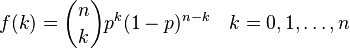
</equation>
Sort of like <xr id="eqn:binom" />, but not really.
References
- ↑ W. H. Sanders. Construction and Solution of Performability Models Based on Stochastic Activity Networks. PhD thesis, University of Michigan, Ann Arbor, Michigan, 1988.
- ↑ 2.0 2.1 S. Derisavi, P. Kemper, and W. H. Sanders. Symbolic state-space exploration and numerical analysis of state-sharing composed models. Linear Algebra and Its Applications, 386:137–166, 15 July 2003.
- ↑ 3.0 3.1 3.2 S. Derisavi, P. Kemper, and W. H. Sanders. Lumping matrix diagram representations of Markov chains. In DSN/PDS, Yokohama, Japan, June/July 2005.
Contents
How to pick the solver[edit]
Möbius provides two types of solvers for obtaining solutions on measures of interest: simulation and numerical solvers. The choice of which type of solvers to use depends on a number of factors. More details on these factors are provided in the sections on simulation (Section 3) and numerical solvers (Section 4).
In general, the simulation solver can be used to solve all models that were built in Möbius, whereas numerical solvers can be used on only those modes that have only exponentially and deterministically distributed actions. In addition, simulation may be used on models that have arbitrarily large state-space descriptions, whereas numerical solvers are limited to models that have finite, small state-space description (that may be held in core memory). Furthermore, simulation may be more useful than numerical solvers for stiff models.
On the other hand, all numerical solvers in Möbius are capable of providing exact solutions (up to machine precision), whereas simulation provides statistically accurate solutions within some user-specifiable confidence interval. The desired accuracy of the computed solutions can be increased without excessive increase in computation time for most numerical solvers, while an increase in accuracy may be quite expensive for simulation. Additionally, full distributions may be computed for results from the numerical solvers, but usually not for results from simulation. Furthermore, for models in which numerical solvers are applicable, detection of rare events incurs no extra costs and requires no special techniques, whereas such computation by simulation is extremely expensive and uses the statistical technique of importance sampling.
Transformers[edit]
Introduction[edit]
Some of the solution techniques within Möbius, such as the simulator, operate directly on the model representation defined using the Atomic and Composed editors described in earlier chapters of the manual. These solvers operator on the model using the Möbius model-level abstract functional interface. There are other solution techniques, specifically the numerical solvers described in the next chapter, which require a different representation of the model as an input. Instead of operating on the high-level model description, numerical solution techniques use a lower-level, state space representation, namely the Markov chain.
Flat State Space Generator[edit]
The flat state space generator1 is used to generate the state space of the discrete-state stochastic process inherent in a model. The state space consists of the set of all states and the transitions between them. Once the state space has been generated, an appropriate analytical solver can be chosen to solve the model, as explained in Section 4.
- 1 This was the only state space generator (SSG) available prior to version 1.6.0 and it was simply called the state space generator. From that version on, it is called the flat state space generator.
While simulation can be applied to models with any underlying stochastic process, numerical solution requires that the model satisfy one of the following properties:
- All timed actions are exponentially distributed (Markov processes).
- All timed actions are deterministic or exponentially distributed, with at most one deterministic action enabled at any time. Furthermore, the firing delay of the deterministic actions may not be state-dependent.
The only restrictions on the use of instantaneous (zero-timed) actions are that the model must begin in a stable state, and the model must be stabilizing and well-specified [1]. It should also be noted that the reactivation predicates (see Section 4.1.1 of Building Models) must preserve the Markov property. In other words, the timed actions in the model must be reactivated so that the firing time distributions depend only on the current state, and not on any past state. That rule pertains only to timed actions with firing delays that are state-dependent.
The flat state space generator consists of a window with two tabs, SSG Info and SSG Output, which are discussed below.
Parameters[edit]
The SSG Info tab (<xr id="fig:ssg_info" />) is presented when you open the interface, and allows you to specify options and edit input to the state space generator.
<figure id="fig:ssg_info">
- The Study Name text box specifies the name of the child study. This box will show the name of the study you selected to be the child when you created the new solver. You can change the child study by typing a new name in the box or clicking the Browse button and selecting the solver child from the list of available studies.
- The Experiment List box displays the list of active experiments in the study, and will be updated upon any changes made through the Experiment Activator button.
- The Experiment Activator button can be used to activate or deactivate experiments defined in the child study, and provides the same functionality as the study editor Experiment Activator described in Section 7.3 of Building Models.
- The Run Name text box specifies the name for a particular run of the state space generator. This field is used to name trace files and output files (see below), and defaults to “Results” when a new solver is created. If no run name is given, the solver name will be used.
- The Build Type pull-down menu is used to choose whether the generator should be run in Optimize or Normal mode. In normal mode, the model is compiled without compiler optimizations, and you can specify various levels of output by changing the trace level, as explained below. This mode is useful for testing or debugging a model, as a text file named Run Name_Expx_trace.txt will be created for each experiment and contain a trace of the generation. In optimize mode, the model is compiled with maximum compiler optimizations, and all trace output is disabled for maximum performance. Running the generator will write over any data from a previous run of the same name, so change the Run Name field if you wish to save output/traces from an earlier run.
- The Build Type pull-down menu is used to choose whether the generator should be run in Optimize or Normal mode. In normal mode, the model is compiled without compiler optimizations, and you can specify various levels of output by changing the trace level, as explained below. This mode is useful for testing or debugging a model, as a text file named
- The Trace Level pull-down menu is enabled only when Normal mode is selected as the Build Type. This feature is useful for debugging purposes, as it allows you to select the amount of detail the generator will produce in the trace. The five options for Trace Level are:
- Level 0: None No detail in the trace. This would produce the same output as if optimize mode were selected.
- Level 1: Action Name For each new state discovered, prints the names of the actions enabled in this state. These are the actions that are fired when all possible next states from the current state are being explored.
- Level 2: Level 1 + State The same as Level 1, with the addition that the current state is printed along with the actions that are enabled in the state.
- Level 3 has not yet been implemented in Möbius.
- Level 4: All The same as Level 2, with the addition that the next states reachable from each state currently being explored are also printed.
- While a higher trace level will produce more detail in the generator trace and aid in debugging a model, it comes at the cost of slower execution time and larger file size.
- The Hash Value text box is used by the hash table data structure, which stores the set of discovered states in the generation algorithm. This number specifies the point at which the hash table is resized. Specifically, it is the ratio of the number of states discovered to the size of the hash table when a resizing2 occurs. The default value of , which means that the hash table is resized when it becomes half full, should suffice for most purposes.
- The Hash Value text box is used by the hash table data structure, which stores the set of discovered states in the generation algorithm. This number specifies the point at which the hash table is resized. Specifically, it is the ratio of the number of states discovered to the size of the hash table when a resizing2 occurs. The default value of
- The Flag Absorbing States checkbox, when selected, will print an alert when an absorbing state is encountered. An absorbing state is one for which there are no next (successor) states.
- The Place Comments in Output checkbox, when selected, will put the user-entered comments in the generator output/trace. If the box is not checked, no comments will appear, regardless of whether any have been entered.
- The Edit Comments button allows you to enter your own comments for a run of the generator. Clicking this button brings up the window shown in <xr id="fig:ssg_commentbox" />. Type any helpful comments in the box and hit OK to save or Cancel to discard the comments. The Clear button will clear all the text from the comment box.
<figure id="fig:ssg_commentbox">
- The Place Comments in Output checkbox, when selected, will put the user-entered comments in the generator output/trace. If the box is not checked, no comments will appear, regardless of whether any have been entered.
- The Experiment List box displays the list of active experiments in the study, and will be updated upon any changes made through the Experiment Activator button.
2 A resizing rehashes and roughly doubles the size of the hash table.
Generation[edit]
Clicking the Start State Space Generation button switches the view to the SSG Output tab and begins the process of generating the state space. The output window appears in <xr id="fig:ssg_output" />.
<figure id="fig:ssg_output">
First the models3 are compiled and the generator is built. For each active experiment, the values of the global variables are printed; if normal mode is being used, information about the trace level and hash table is also displayed. Then the state space is generated for the experiment. While it is being generated, the States Generated box and progress bar at the bottom of the dialog indicate the number of states that have been discovered. This number is updated once for every 1,000 states generated and when generation is complete. At any time, you may use the Stop button to terminate the run. A text file named Run Name_output.txt will be created. It will mirror the data output in the GUI.
- 3 Here models refers to the atomic/composed models, performance variable, and study.
A final remark is in order about the notion of state during generation of the state space of the stochastic process. In Möbius, a state is defined as the values of the state variables along with the impulse reward (see Section 6.1.1 of Building Models) associated with the action whose firing led to that state. Therefore, for a model on which impulse rewards have been defined, if two different actions may fire in a given state and lead to the same next state, they give rise to two unique states in the state space. The reason is that when impulse rewards are defined, the state space generator must store information about the last action fired. The result is a larger state space for models on which impulse rewards have been defined. It is important to realize this when analyzing the size of the generated state space.
Command line options[edit]
The flat state space generator is usually run from the GUI. However, since the models are compiled and linked with the generator libraries to form an executable, the generator can also be run from the command line (e.g., from a system shell/terminal window). The executable is found in the directory
- Möbius Project Root/Project Name/Solver/Solver Name/
-
and is named Solver NameGen_Arch[_debug], where Arch is the system architecture (Windows, Linux, or Solaris) and _debug is appended if you build the flat state space generator in normal mode. The command line options and their arguments are as follows:
-P experimentfilepath
- Place the created experiment files in the directory specified by experimentfilepath. This argument can be a relative path. By default, the experiment files will be placed in the current directory, but you can specify a path using the option “-E.”
-N experimentname
- Use experimentname to name the experiment files created. These files will have extensions .arm or .var, and will be placed in the directory specified by the “-E” option.
-B experimentnumber
- Generate the state space for the experiment numbered experimentnumber, with the first experiment having number 0. For example, use “-B1” to run the second experiment (e.g., Experiment_2). Defaults to 0.
-h hash_value
- Use hash_value as the hash value described above. Defaults to 0.5.
-a
- Flag absorbing states.
-F filetype[1-6]
- Use filetype as the format for the experiment file. The only filetype currently supported in the flat state space generator is “-F1,” or row ASCII format, which is also the default option. Other file formats may be available in future versions.
-e, -s db_entity, db_macserver
- These are internal options for interaction with the database. You can safely ignore them.
-l trace_level[0-4]
- Use trace_level as the trace level described above. Only applies when you are running the debug executable.
-t tracefilename
- Create a trace file named tracefilename as output. If this option is not specified, output is directed to the standard output stream.
Example: ssgGen_Windows_debug -E. -B0 -l4 -ttrace.txt
- Solver Name is ssg
-
- Arch is Windows
-
This command will generate the state space for the first experiment (Experiment_1) with trace level 4, place the experiment files in the current directory, and create a trace file named trace.txt.
Symbolic State Space Generator[edit]
The symbolic state space generator (symbolic SSG) is a component that was added to the Möbius tool for version 1.6.0. In this chapter, we first introduce this component, discuss its advantages and limitations, and describe how to use it in an efficient way. Then, we will explain how to fill up each of the input parameters of its corresponding GUI editor. The different phases of the state space generation will be briefly described. Finally, we will provide instructions on how to run the symbolic SSG from the command line. For more details on the inner workings of the symbolic SSG, please see [2] [3].
Introduction[edit]
In solving a model using numerical solution, a modeler must first run a state space generator on the model to build a representation of the stochastic process underlying the model, and then use a numerical solver to compute the measures (s)he is interested in.
A numerical solution algorithm needs data structures to represent two essential entities in the memory: the stochastic process (input) and one or more probability distribution vectors (output). The stochastic process is generated by a state space generator. In this chapter, we only consider stochastic processes that are continuous time Markov chains (CTMCs), and can therefore be represented by state transition rate matrices whose entries are the rates of exponentially distributed timed transitions from one state to another.
In many numerical solvers, sparse matrix representation and arrays are respectively used to represent the process and the probability vector(s). In such a design of data structures, the stochastic process represented by a sparse matrix almost always takes more memory space than the probability vectors.
A problem arises when the model under study is so large that the memory requirement of the two data structures exceeds the amount of memory available on a computer. For example, to analyze a model with ten million states for a specific point of time using the transient solver (TRS) and the data structures mentioned above, at least bytes MB to bytes MB (depending on the model) of RAM are needed, assuming that each state leads to 10 to 20 other (successor) states and each floating-point number requires 8 bytes of storage.
That problem has stimulated a lot of research looking for more “practical” data structures, i.e., more compact (with smaller space requirements) data structures that do not incur too much time overhead. The most practical data structure that virtually all numerical solvers (including ones in Möbius) use to represent probability distribution vectors is simply an array. Efforts by researchers to design better ones have failed so far.
However, there has been a lot of successful research on design of data structures for the representation of the state transition matrix. In particular, symbolic data structures (hence the name symbolic SSG) are widely used nowadays to store state transition matrices in a very compact manner. As opposed to sparse matrix representation, symbolic data structures do not have space requirements proportional to the number of nonzero entries. In virtually all cases, they take up orders of magnitude less space than their sparse representation counterparts. This extremely low space requirement enables the modeler to numerically solve models that are much larger than was previously possible. For example, to do the same analysis we mentioned above, we only need about 100 MB of RAM using symbolic data structures. Because of the concept behind symbolic data structures and the way they are constructed, we see their benefits only in composed models, especially those consisting of atomic models of appropriate sizes; more information on this will be provided later in the section.
The major price a modeler has to pay is overhead in speed. Based on our measurements, when the symbolic SSG is used to generate the state space, numerical solution is expected to be about 3 to 10 times slower than it would be for the flat SSG. Notice that slowdown is not related to the state space generation itself. In fact, in virtually all cases, the symbolic SSG is faster than the flat SSG; in some cases it may be several times faster.
The symbolic SSG utilizes three types of symbolic data structures to represent the required entities. It uses MDDs (Multi-valued Decision Diagrams) for the set of reachable states, MxDs (Matrix Diagrams) for the state transition rate matrices, and MTMDDs (Multi-Terminal MDDs) for the values of the performance variables in each reachable state.
The symbolic SSG utilizes two types of lumping algorithm. Lumping is a technique in which states of a CTMC that are behaviorally “equivalent” are lumped together and replaced by a single state. Therefore, the number of states of a “lumped” CTMC is always equal to or smaller than the number of states of the original CTMC. The performance variables computed from a lumped CTMC are exactly the same as the performance variables computed from the original one. That means that we save on both time and space if we solve a smaller lumped CTMC rather than the original one. For example, models that consist of a number of equal parts or components have a potential for lumping that reduces the size of the state space significantly.
The first lumping technique is called model-level lumping, in which the symmetry of a Replicate/Join model is exploited as explained in Section 5.1.1 of Building Models to reduce the size of the state space. That lumping technique has been part of the symbolic SSG from the beginning.
The second lumping technique that has been added to symbolic SSG in version 1.8.0 is called compositional lumping. In compositional lumping, the lumping algorithm is applied to individual components (atomic models in the Möbius context) of a compositional model, whereas in state-level lumping the algorithm is applied to the overall CTMC generated from the model. In fact, that is the main advantage of the compositional lumping technique over state-level lumping; it is applied on CTMCs of components that are much smaller than the CTMCs of the whole model. That advantage means that, in general, compositional lumping algorithms require less time and memory space for their operation. Möbius supports ordinary compositional lumping. See [3] for more information.
To summarize, the symbolic SSG uses compact data structures to represent the state transition rate matrix of Markov chains such that it devotes most of the available RAM to the storage of the probability distribution vector(s). If possible, it uses model-level and compositional lumping algorithms to reduce the size of the state space of the CTMC that needs to be solved in order to compute the desired performance variables. That makes it possible for the modeler to numerically analyze models that are orders of magnitude larger than was previously possible using flat SSG and sparse matrix representation.
Limitations[edit]
As we mentioned above, speed is the major price we pay in using symbolic data structures. Moreover, there are a number of conditions that have to be satisfied before we can use the symbolic SSG:
- The stochastic process underlying a model has to be Markov. Therefore, only exponential and immediate (i.e., zero-timed) transitions are allowed.
- If the model under study is a composed one, immediate transitions must not affect or be affected by shared state variables.
- The reward model must not have impulse reward definitions.
- The starting state has to be stable (not vanishing), i.e., no immediate transition should be enabled in the starting state.
If any of the above conditions is not met for a model, the symbolic SSG is not usable, and its GUI shows a message indicating the unmet condition(s).
Finally, when using the iterative steady state solver, it is not possible to use the SOR (Successive Over Relaxation) variant with state spaces that are generated using symbolic SSG. Instead, the Jacobi variant should be used. The reason is that the symbolic data structure constructed by the SSG does not provide the elements of the state transition matrix in any specific order (see Section 4.3.3).
Tips on efficient use[edit]
The time and space efficiency of the symbolic SSG can vary widely depending on the way the model is built. We have observed up to one order of magnitude of speed difference among a number of composed models that result in the same underlying Markov chain. Theoretically speaking, even larger differences are possible. Here are two guidelines that will help modelers construct their models in a way that increases the performance of the symbolic SSG:
- Do not use symbolic SSG for atomic models, especially large atomic models. Not only does it not give any better performance, it drastically reduces both time and space efficiency of state space generation and numerical analysis. For those types of models, simply use the flat state space generator.
- Try to decompose the complete model into atomic models such that each of them has roughly 3 to 50 states. In the general case, it is impossible to estimate how many states an atomic model has. However, the modeler can sometimes make an estimation. Above 50 states, the larger the atomic models’ state spaces are, the more the state space generation performance will be negatively affected.
Parameters[edit]
The SSG Info tab (<xr id="fig:symssg_info" />) is presented when you open the interface, and allows you to specify options and edit input to the symbolic state space generator.
<figure id="fig:symssg_info">
- The Study Name text box specifies the name of the child study. This box will show the name of the study you identified as the child when you created the symbolic SSG. You can change the child study by typing a new name in the box or clicking the Browse button and selecting the solver child from the list of available studies.
- The Experiment List box displays the list of active experiments in the study, and will be updated in response to any changes made through the Experiment Activator button.
- The Experiment Activator button can be used to activate or deactivate experiments defined in the child study, and provides the same functionality as the study editor Experiment Activator described in Section 7.3 of Building Models.
- The Run Name text box specifies the name for a particular run of the symbolic state space generator. This field is used to name trace files and output files (see below), and defaults to “Results” when a new symbolic SSG is created. If no run name is given, the symbolic SSG name will be used.
- The Build Type pull-down menu is used to choose whether the generator should be run in Optimize or Normal mode. In normal mode, the model is compiled without compiler optimizations, and you can specify various levels of output by changing the trace level, as explained below. This mode is useful for testing or debugging a model, as a text file named Run Name_Expx_trace.txt will be created for each experiment and contain a trace of the generation. In optimize mode, the model is compiled with maximum compiler optimizations, and all trace output is disabled for maximum performance. Running the generator will write over any data from a previous run of the same name, so change the Run Name field if you wish to save output/traces from an earlier run.
- The Build Type pull-down menu is used to choose whether the generator should be run in Optimize or Normal mode. In normal mode, the model is compiled without compiler optimizations, and you can specify various levels of output by changing the trace level, as explained below. This mode is useful for testing or debugging a model, as a text file named
- The Trace Level pull-down menu is enabled only when Normal mode is selected as the Build Type. This feature is useful for debugging purposes, as it allows you to select the amount of detail the generator will produce in the trace. The two options for Trace Level are:
- Level 0: None The processing time for each phase of the generation is printed out (see the next section for more on generation phases). Moreover, the numbers of unlumped and lumped states are also shown. The ouput is the same as it would be if optimize mode were selected.
- Level 1: Verbose This includes everything printed in Level 0, plus detailed information about the symbolic data structures, such as the number of levels, the size of the nodes in each level, the final number of nodes, the maximum number of nodes during the runtime, and the number of firings of local and global actions.
- The symbolic SSG does not produce a great deal of debugging information; therefore, you will not notice much difference between the execution times of the two different trace levels.
- The numbers entered in the MDD Unique Table Size and MxD Unique Table Size text boxes are used by the MDD and MxD data structures. They are the sizes of the hash tables used to store all the unique nodes of the MDD and MxD data structures, respectively. Their default values are 50,000 and 10,000, and their minimum values are 5,000 and 1,000, respectively.
- There is no clear-cut set of rules on how to set these numbers. The default values should be appropriate for most models. For extremely large models for which the state space generation takes much more than an hour, double or quadruple the default values. Increasing the values above a certain value deteriorates the performance of the SSG algorithm.
- The Enable Compositional Lumping checkbox, when selected, activates the compositional lumping algorithm, which for some models (but not all of them) reduces the size of the CTMC that needs to be solved. Although enabling the algorithm increases the running time of the state space generation, in some cases, it leads to significant reduction in the numerical solution time.
- The Place Comments in Output checkbox, when selected, will put the user-entered comments in the generator output/trace. If the box is not checked, no comments will appear, regardless of whether any have been entered.
- The Edit Comments button allows you to enter your own comments for a run of the generator. Clicking this button brings up the window shown in <xr id="fig:ssg_commentbox" />. Type any helpful comments in the box and hit OK to save or Cancel to discard the comments. The Clear button will clear all the text from the comment box.
Generation[edit]
Clicking the Start State Space Generation button switches the view to the SSG Output tab and begins the process of generating the state space. Snapshots of the output window in different phases of the generation appear in <xr id="fig:symssg_output" />.
<figure id="fig:symssg_output">
| <subfigure></subfigure>
|
<subfigure></subfigure>
|
| (a) Just after starting. | (b) Performing phase 6 (compositional lumping is enabled). |
As for the flat state space generator, the generation begins by compiling the models4 and building the generator. For each active experiment, the values of the global variables are printed.
- 4 Here models refers to the atomic/composed models, performance variable, and study.
The state space is then generated for the experiment in six phases if compositional lumping is enabled, and in five phases otherwise. Two progress bars at the bottom of the dialog show the amount of completed work. The Overall progress bar indicates which phase is in progress and the overall progress of the generation, and the Phase progress bar indicates the progress of each phase of the generation. The amount of time taken to complete each phase is printed after the phase is finished. At any time, you may use the Stop button to terminate the run. A text file named Run Name_output.txt will be created. It will mirror the data output in the GUI.
The 6 phases are:
- The unlumped state space is generated in the form of an MDD data structure in a number of iterations (see Section 5.1.1 of Building Models for definitions of lumped and unlumped state spaces). The total number of iterations depends on the model and is not known in advance. After each iteration is complete, the Phase progress bar shows the iteration number and the number of unlumped states that have been explored so far. When this phase is completed, the total number of explored unlumped states is printed. Phases 1, 3, and 6 are often the most time-consuming phases of the generation process.
- The MxD data structure representing the state transition rate matrix of the unlumped CTMC is built in this phase. This phase is usually completed very quickly.
- In this phase and the following one, lumping algorithms are applied on the state space to reduce the size of the CTMC that needs to be solved to compute the desired performance variables. In this phase, the compositional lumping algorithm is applied on the unlumped state space. The size of the state space lumped by the compositional lumping algorithm is printed out at the end of the step. This phase is performed in two subphases. In the first one, the initial partition for each atomic model is computed based on the values of the performance variables. In the second subphase, which is based on an efficient partition-refinement algorithm[3], the initial partition is refined repeatedly to compute the lumped state space for each atomic model. Virtually for all models, the second subphase is much faster than the first subphase.
- In this phase, the model-level lumping induced by Replicate/Join operators is performed. The size of the state space after compositional and model-level lumping is printed out at the end of this step. This phase usually takes the least amount of time of all the phases.
- For each of the performance variables defined on the model, one MTMDD symbolic data structure is built. This data structure gives the value of that performance variable for each state of the lumped state space.
- The “mapping” MDD, a special type of the MDD data structure, is constructed in this phase[2]. This phase has two subphases. In the first, the set of states of the mapping MDD is computed; during this process, the progress bars are not updated because the cardinality of the set is not known yet. In the second subphase, the mapping MDD construction actually starts. While the mapping MDD is being built, the Phase progress bar shows the number of states of the mapping MDD built so far, the total number of states of the mapping MDD, and the fraction of the phase that has been completed. The Overall progress bar is also updated accordingly.
Command line options[edit]
The symbolic state space generator is usually run from the GUI. However, since the models are compiled and linked with the generator libraries to form an executable, the generator can also be run from the command line (e.g., from a system shell/terminal window). The executable is found in the directory
- Möbius Project Root/Project Name/Solver/Solver Name/
-
and is named Solver NameSymGen_Arch[_debug], where Arch is the system architecture (Windows, Linux, or Solaris) and _debug is appended if you build the symbolic state space generator in normal mode. The command line options and their arguments are as follows:
-P experimentfilepath
- Same as the flat state space generator. For more details, refer to Section 2.2.3.
-N experimentname
- Same as the flat state space generator. For more details, refer to Section 2.2.3.
-B experimentnumber
- Generate the state space for the experiment numbered experimentnumber, with the first experiment having number 0. For example, use “-B1” to run the second experiment (e.g., Experiment_2). Defaults to 0.
-c
- Enables the compositional lumping algorithm, which is disabled by default.
-e, -s db_entity, db_macserver
- These are internal options for interaction with the database. You can safely ignore them.
-l trace_level[0-1]
- Use trace_level as the trace level described above. Only applies when you are running the debug executable.
-t tracefilename
- Create a trace file named tracefilename as output. If this option is not specified, output is directed to the standard output stream.
-d MDD_Utable_size, union_cache_size, local_exploration_cache_size, MxD_Utable_size, submat_cache_size, add_cache_size
- These are the different parameters for the symbolic data structures. They should follow the -d option in the form of a comma-separated list of non-negative numbers. The numbers in parentheses are the default value and the minimum value enforced by the symbolic SSG.
- MDD_Utable_size The size of the unique table of the MDD (50,000 and 1,000)
- union_cache_size The cache size of the union operation of the MDD (10,000 and 500)
- local_exploration_cache_size The cache size of the local state space exploration operation of the MDD (10,000 and 500)
- MxD_Utable_size The size of the unique table of the MD (10,000 and 500)
- submat_cache_size The cache size of the submatrix operation of the MD (5,000 and 100)
- add_cache_size The cache size of the add operation of the MD (5,000 and 100)
- This command line option is optional. If it is not given, the default values will be used. If the option is present and the value for a parameter is zero or not given (i.e., there is no character between two consecutive commas) the default value for that parameter is used.
Example: sssgSymGen_Linux_debug -E. -B0 -l1 -ttrace.txt
-d 50000,,10000,0,5000,5000
- Solver Name is sssg
-
- Arch is Linux
-
This command will generate the state space for the first experiment (Experiment_1) with trace level 1, place the experiment files in the current directory, and create a trace file named trace.txt. All parameters for the symbolic data structures except union_cache_size and MD_Utable_size are given by the user via the -d option. For those two parameters the default values are used.
Simulator[edit]
The simulator can be used to solve models using discrete event simulation. It takes the model and parameters specified by a study, links the libraries for those models together with the simulator library, and runs the executable. The simulator can be used to solve any model specified in Möbius, and can be used to solve for transient and steady state results.
Simulation Parameters[edit]
The Simulation Parameters tab on the Simulator editor allows you to specify all of the simulation parameters and is shown in <xr id="fig:sim_parameters" />.
<figure id="fig:sim_parameters">
The parameters on the page can be roughly broken down into four categories that proceed down the tab.
- Study and experiment selection
- Simulation execution parameters
- Compilation options
- Checkboxes
Study and experiment selection[edit]
The top of the tab starts with the Current Study field, which contains the name of the study to be solved. The study is initially set when you create the simulation, and you are prompted to specify the solver child. You can change the study by typing a new study name into the field, or by clicking the Browse button. If you click on the Browse button, the Select Solver Child window will pop up. It shows all of the studies and prompts you to select one.
The Experiment Activator button opens a pop-up window (shown in <xr id="fig:sim_experiment" />) to allow you to view and select the experiments in the study. Recall that all global variable values are assigned in the study, and that each unique set of assignments is called an experiment. The pop-up window shows all of the experiments in the study, the global variable values for each experiment, and the experiments that have been activated in this simulation so that they will be solved. You can activate or deactivate an experiment by checking the box above the experiment. You can activate or deactivate all experiments by clicking on the Activate All or Deactivate All buttons.
<figure id="fig:sim_experiment">
Simulation execution parameters[edit]
The next set of parameters affect the execution of the simulation.
- The radio boxes under Simulation Type specify whether the model solution should be a steady state solution or a terminating solution. If the model contains transient rewards, the Terminating Simulation option will be enabled, and if the model contains steady state rewards, the Steady State Simulation option will be enabled. If all the rewards are either transient or steady state, only one option will be enabled, and it will be selected by default.
- The pull-down menu Random Number Generator is used to select the pseudo-random number generator to use in the solution. The default option is the Lagged Fibonacci random number generator, but the Tauseworthe random number generator can be used.
- The Random Number Seed field specifies the seed for the pseudo-random number generator. The default value is 31,415, but any value can be used. Once the seed has been specified, the sequence of numbers is deterministic. Multiple simulations with the same random number seed should generate the same results5.
- The Maximum Batches field specifies the maximum number of batches (in steady state simulation) or replicas (in transient simulation) that the simulator will run. The simulator will run several batches or replicas to generate data for the confidence intervals. The simulator will continue to run more batches or replicas until all of the results have converged to their specified confidence intervals. This option will terminate the simulation if the simulator has run the maximum number of batches, even if not all of the reward variables have converged to their specified confidence intervals.
- The Minimum Batches field specifies the minimum number of batches (in steady state simulation) or replicas (in transient simulation) that the simulator will run. The simulator will run several batches or replicas to generate data for the confidence intervals. The simulator will continue to run more batches or replicas until all of the results have converged to their specified confidence intervals. This option ensures that the simulator will run at least the minimum number of batches or replicas before finishing. This is useful in simulating rare events, for which the model’s reward variables may appear to converge too early if no rare events have occurred.
- The Number of Batches per Data update field specifies how many batches or replicas the simulation executables should complete before sending those results back to the editor. If the simulation is run on multiple machines, each machine will send an update after simulating the specified number of batches or replicas.
- The Number of Batches per Display update field specifies how many batches or replicas should be received by the editor before it updates the user interface. A low number will provide the most up-to-date data, but can cause the user interface to use too many resources. A larger number will reduce the load created by the user interface, but will also provide fewer updates. In general, this number should always be greater than or equal to the number specified in Number of Batches per update.
5 The simulator is multi-threaded and can be distributed. Due to timing variations in a distributed environment, the results will not necessarily be identical when an experiment is simulated multiple times with the same random number seed, even though the random number sequences will be identical.
Compilation options[edit]
The next set of options control how the simulation is compiled and run, allowing for optimizations, trace output, and specification of the run name.
- The Build Type pull-down menu allows you to set the model to run in either optimized or normal mode. In normal mode, the model is compiled without compiler optimizations, and it is possible to specify various levels of output by changing the trace level. In optimized mode, the model is compiled with compiler optimizations, and all trace output is disabled for maximum performance. You would normally use normal mode for testing a model and making sure it is behaving properly, while you would use optimized mode for production simulations.
- The Build Architecture pull-down menu allows you to set the model to execute in either 32-bit or 64-bit mode. On 32-bit machines (or machines running a 32-bit operating system), this drop down menu will be disabled and only 32-bit execution is available.
- The Trace Level pull-down menu allows you to set the level of detail included in a trace of the simulation. The trace includes key information about the evolution of the simulation in a text file, which can be used to debug a model. The available trace levels are:
- – 0: No Output: No trace file is generated.
- – 1: Firing Time and Activity Name: This option will include the simulation time of every activity completion, and the name of the activity that fired.
- – 2: Level 1 plus Minimal State: This level adds some relevant state information from the time of the activity firing to the previous level’s activity firing times and names. Specifically, it shows the values of state variables that are either part of the enabling conditions for the activity, or part of the state affected by the activity.
- – 3: Level 1 plus All State: This level prints out all of the state information at every activity firing, in addition to the name of the activity and the time it fires.
- – 4: All: This level prints out all of the information from the previous levels plus more data on which activities are enabled, become enabled, or become disabled when an activity fires.
- The trace-level options can generate useful information that you can use to understand the behavior of your models. However, it can also generate more information that you want. Generally, trace output is only used with a small number of batches.
- The Run name field specifies the name for this run of the simulation. This is used to name trace files and output files. Change the run name any time you want to save existing results from a previous run of the simulator. Otherwise, the new results will overwrite any existing results.
Checkboxes[edit]
The last set of options are set using checkboxes. Most of them control the output of the simulator, while one of them controls the variance calculation.
- Store simulator console output to file stores all of the output from the editor display to a file.
- The Store observations to ASCII .csv file option can be used to save the raw simulation results to a file for later use. Again, this option is useful if you are running remote simulations over a low-bandwidth connection, because you can access the observations at a later time to get the results of the simulation. The option stores the observations in an ASCII file format. ASCII is human-readable, and can also be loaded into tools like Excel for custom analysis.
- The Store observations to binary .dat file option can be used to save the raw simulation results to a file for later use. This option is useful if you are running remote simulations over a low-bandwidth connection. You can access the observations at a later time to get the results of the simulation. The option stores the observations in a binary file, which should be smaller than the ASCII file the other option would have produced. The binary files are used by Möbius for off-line processing (see Section 3.3.2).
- There used to be a checkbox in the Simulation Parameters tab called Use Jackknife Variance Calculation that made the simulator use the advanced jackknife method of variance calculation. In Möbius 1.8.0 and later, the method is always used; therefore, the checkbox has been removed.
Network Setup[edit]
Use the Network Setup tab, shown in <xr id="fig:sim_network" />, to select the computers on which the simulation will be run. You can parallelize simulations by executing multiple replicas of the simulation on different machines at the same time, with near linear speed-up in solution time. On the left of the tab is the Available Systems list of machines or groups of machines that can be used in the solution of the model. You can select one or more machines for use by selecting their names in the list, and then clicking on the >> button. Clicking on the button will transfer all of the selected machines to the Selected Systems list. You can deselect machines in the same manner, by selecting their names in the Selected Systems list and clicking on the << button.
<figure id="fig:sim_network">
You can edit the list of available systems by clicking on the Edit Machine/Group Info button. Clicking on the button opens the Network Machine and Group Settings dialog, which is described in Section ??.
The Number of Processors per Experiment drop-down menu allows you to select the number of processors to use per experiment. The simulator can assign multiple machines to simulate the same experiment, and each experiment will be assigned a number of machines no greater than the specified number. Machines will be assigned to the lowest-numbered experiment that has not yet been solved and that has fewer than the specified number of machines.
The Maximize Processor Usage checkbox overrides the Number of Processors per Experiment setting. If the Maximize Processor Usage option is enabled, the simulator will distribute experiments to all the machines, such that each experiment is running on a similar number of machines. When an experiment finishes, the machines that were assigned to it are then reassigned to the other experiments. In that way, all of the experiments are solved as quickly as possible.
Running Simulation[edit]
The Run Simulation tab, shown in <xr id="fig:sim_run" />, is used to start and stop the simulator. As the simulation is being compiled and run, messages are produced and are shown in the Simulation Status area. The information includes the name of all the files being compiled and linked, and indicates when the execution of the simulation begins.
<figure id="fig:sim_run">
On the bottom of the tab are a couple of check boxes and a series of buttons to control the running of the simulation. The checkboxes Skip compile and Force compile control whether the underlying files are compiled before starting the simulations. By default, the simulator editor will recompile the minimum set of files before starting the simulations for the first time if neither checkbox is checked.
There are two modes for generating simulator results. The first mode is on-line, in which the simulation executables are run and the results are computed and displayed by the editor as the solution converges. The second mode is off-line. There are two steps in off-line simulation: the first step is the launch of the simulation executables with the binary output file option enabled, and the second step is the processing of the binary output files when the simulator processes have completed. The two modes are discussed in the following sections.
On-line simulation[edit]
The Start Simulation button starts the simulator. Any files that should be recompiled are recompiled, and experiments are assigned to the selected machines.
The Stop Simulation button will stop a running simulation. It will stop all of the simulations started on remote machines, and finish any remaining result computation.
The Client Information dialog, shown in <xr id="fig:sim_clientinfo" />, is used to check the status of a client machine during solution. The Client Information window will pop up with a list of client machines used in this simulation. When you double-click on any of the system names, the Client Status window, shown in <xr id="fig:sim_clientstatus" />, will pop up to provide the name of the system, the architectures, and the operating system.
<figure id="fig:sim_clientinfo">
<figure id="fig:sim_clientstatus">
Off-line simulation[edit]
The Process Binary File button allows you to process a binary output file that was generated if you checked the Store observations to binary .dat file option, as described in Section 3.1.4. When you press the button, a file browser will open to allow you to select the appropriate binary data output file(s). Once you have selected the files, Möbius reads them and processes the data as if the simulation was running on-line, and displays the results after all data has been read.
Binary data files can be generated through multiple simulation runs. You can launch runs with the Möbius simulation editor or launch the simulation executable directly via the command line.
One reason to use the off-line processing capability is to generate solutions without having to run the Möbius graphical interface. You can launch jobs on the command line (directly or via user-constructed command line scripts), collect the results, and transfer them to a machine with graphical access on which the data files can be processed to compute the results.
Another reason to use off-line processing is to generate more simulation replications than could be generated in one session. Repeated executions of the simulator (using a unique random seed and run name each time) will produce multiple sets of data files. These files can be processed together at one time to generate results based on all the runs.
Simulation Info[edit]
The Simulation Info tab displays the results for the experiments as they become available, and is shown in <xr id="fig:sim_results" />. At the top left of the tab is the list of all the enabled experiments and their statuses. The Status column indicates whether the experiment has not started, is running, or has completed. The # CPUs column indicates how many processors are currently assigned to the given experiment, and the Batches column indicates how many batches or replicas of that experiment have completed and been reported back to the user interface. You can select an experiment by clicking on its row in the table. Selecting the experiment in the list updates the Selected Experiment display in the lower half of the window. The Selected Experiment display shows the simulation progress by reporting the number of replications computed and showing the mean and variance values and confidence intervals for each reward variable. When the result converges so that the computed confidence interval is within the tolerances specified in the Simulation panel of the Performance Variable Editor (see Section 6.1.6 of Building Models), the color of the reward variable row changes from red to blue.
<figure id="fig:sim_results">
There are three buttons to the right of the experiment list:
- The Terminate Selected Experiment button stops the solution of the currently selected experiment. All machines that are simulating that experiment stop doing so, and are reassigned.
- The Terminate All Experiments button stops the solution of all the experiments. The simulator receives the final updates and displays the final results.
- The Show Results button opens the Simulation Results window, which is discussed in the next section.
Simulation Results[edit]
The results of the simulation are displayed in the Simulation Results tab when the simulation finishes or the user clicks on the Show Results button of the Simulation Info tab. The window displays the human-readable text output created by the simulator. The file includes all of the parameters for the model, all of the experiments, and all of the results. In addition to the human-readable output, a comma-separated-value file (.csv) is also created. The csv file is designed to be simple to import into third-party plotting and analysis tools (such as Excel).
Command Line Options[edit]
The simulator is normally run from the simulator editor. However, it can also be run from the command line. The simulator executable resides in the project tree, in a path following this pattern: Möbius Project Root/Project Name/Solver/Solver Name/. It can be run with the command line options listed in <xr id="tab:command_options" />. These options will be shown if you execute the simulator on the command line, without any options.
<figtable id="tab:command_options">
| Option | Description |
|---|---|
Möbius
Möbius[edit]
Motivation[edit]
Solution[edit]
Graph
Edit Möbius Documentation
“” –
<equation id="eqn:binom" shownumber>
</equation>
Sort of like <xr id="eqn:binom" />, but not really.
References[edit]
- ↑ W. H. Sanders. Construction and Solution of Performability Models Based on Stochastic Activity Networks. PhD thesis, University of Michigan, Ann Arbor, Michigan, 1988.
- ↑ 2.0 2.1 S. Derisavi, P. Kemper, and W. H. Sanders. Symbolic state-space exploration and numerical analysis of state-sharing composed models. Linear Algebra and Its Applications, 386:137–166, 15 July 2003.
- ↑ 3.0 3.1 3.2 S. Derisavi, P. Kemper, and W. H. Sanders. Lumping matrix diagram representations of Markov chains. In DSN/PDS, Yokohama, Japan, June/July 2005.